Linear Programming Lecture Notes - Penn State Personal Web Server

2. Graphically Solving Linear Programs Problems with Two Variables
(Bounded Case)
Linear Programs (LP’s) with two variables can be solved graphically by plotting the
feasible region along with the level curves of the objective function. We will show that we
can find a point in the feasible region that maximizes the objective function using the level
curves of the objective function. We illustrate the method first using the problem from
Example 2.3.
Example 2.4 (Continuation of Example 2.3). Let’s continue the example of the Toy
Maker begin in Example 2.3. To solve the linear programming problem graphically, begin
by drawing the feasible region. This is shown in the blue shaded region of Figure 2.1.
3x1 + x2 = 120
3x1 + x2 ≤ 120
x1 +2x2 ≤ 160
∇(7x1 +6x2)
x1 ≤ 35
x1 ≥ 0
x2 ≥ 0
x1 = 35
x1 +2x2 = 160
(x ∗ 1,x ∗ 2) = (16, 72)
3x1 + x2 ≤ 120
x1 +2x2 ≤ 160
x1 ≤ 35
x1 ≥ 0
x2 ≥ 0
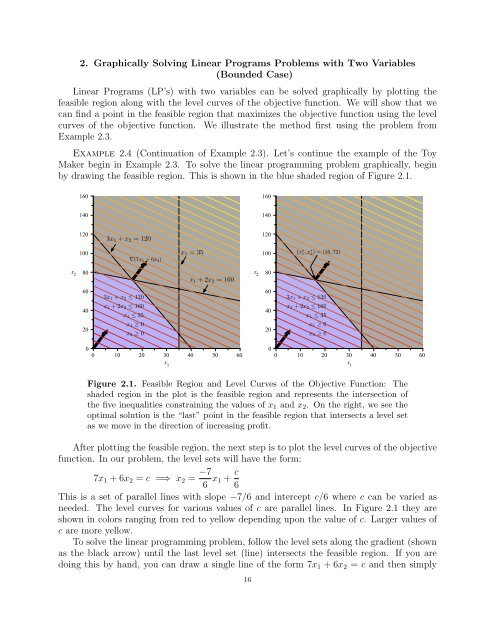
Figure 2.1. Feasible Region and Level Curves of the Objective Function: The
shaded region in the plot is the feasible region and represents the intersection of
the five inequalities constraining the values of x1 and x2. On the right, we see the
optimal solution is the “last” point in the feasible region that intersects a level set
as we move in the direction of increasing profit.
After plotting the feasible region, the next step is to plot the level curves of the objective
function. In our problem, the level sets will have the form:
7x1 + 6x2 = c =⇒ x2 = −7
6 x1 + c
6
This is a set of parallel lines with slope −7/6 and intercept c/6 where c can be varied as
needed. The level curves for various values of c are parallel lines. In Figure 2.1 they are
shown in colors ranging from red to yellow depending upon the value of c. Larger values of
c are more yellow.
To solve the linear programming problem, follow the level sets along the gradient (shown
as the black arrow) until the last level set (line) intersects the feasible region. If you are
doing this by hand, you can draw a single line of the form 7x1 + 6x2 = c and then simply
16