Linear Programming Lecture Notes - Penn State Personal Web Server

More documents

Recommendations

Info

Suppose we choose s4 as the leaving variable. Then our tableau will become: ⎡ ⎤ z x1 x2 s1 s2 s3 s4 RHS MRT (s1) z ⎢ 1 0 0 −14/5 0 0 44/5 544 ⎥ x1 ⎢ (5.47) ⎢ 0 1 0 4/5 0 0 −4/5 16 ⎥ 20 x2 ⎢ 0 0 1 −7/5 0 0 12/5 72 ⎥ − s2 ⎣ 0 0 0 2 1 0 −4 0 ⎦ 0 s3 0 0 0 −4/5 0 1 4/5 19 − We now observe two things: (1) One of the basic variables (s2) is zero, even though it is basic. This is the indicator of degeneracy at an extreme point. (2) The reduced cost of s1 is negative, indicating that s1 should enter the basis. If we choose s1 as an entering variable, then using the minimum ratio test, we will choose s2 as the leaving variable (by the minimum ratio test) 2 . Then the tableau becomes: (5.48) z x1 x2 s1 ⎡ z ⎢ 1 ⎢ 0 ⎢ 0 ⎣ 0 x1 0 1 0 0 x2 0 0 1 0 s1 0 0 0 1 s2 7/5 −2/5 7/10 1/2 s3 0 0 0 0 s4 16/5 4/5 −2/5 −2 ⎤ RHS 544 ⎥ 16 ⎥ 72 ⎥ 0 ⎦ 0 0 0 0 2/5 1 −4/5 19 s3 Notice the objective function value cBB −1 b has not changed, because we really have not moved to a new extreme point. We have simply changed from one representation of the degenerate extreme point to another. This was to be expected, the fact that the minimum ratio was zero showed that we could not increase s1 and maintain feasibility. As such s1 = 0 in the new basic feasible solution. The reduced cost vector cBB −1 N − cN has changed and we could now terminate the simplex method. Theorem 5.16. Consider Problem P (our linear programming problem). Let B ∈ R m×m be a basis matrix corresponding to some set of basic variables xB. Let b = B −1 b. If bj = 0 for some j = 1, . . . , m, then xB = b and xN = 0 is a degenerate extreme point of the feasible region of Problem P . Proof. At any basic feasible solutions we have chosen m variables as basic. This basic feasible solution satisfies BxB = b and thus provides m binding constraints. The remaining variables are chosen as non-basic and set to zero, thus xN = 0, which provides n−m binding constraints on the non-negativity constraints (i.e., x ≥ 0). If there is a basic variable that is zero, then an extra non-negativity constraint is binding at that extreme point. Thus n + 1 constraints are binding and, by definition, the extreme point must be degenerate. 7.1. The Simplex Algorithm and Convergence. Using the work we’ve done in this chapter, we can now state the following implementation of the Simplex algorithm in matrix form. 2 The minimum ratio test still applies when bj = 0. In this case, we will remain at the same extreme point. 88
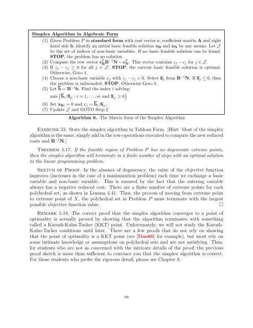
Simplex Algorithm in Algebraic Form (1) Given Problem P in standard form with cost vector c, coefficient matrix A and right hand side b, identify an initial basic feasible solution xB and xN by any means. Let J be the set of indices of non-basic variables. If no basic feasible solution can be found, STOP, the problem has no solution. (2) Compute the row vector c T B B−1 N − c T N . This vector contains zj − cj for j ∈ J . (3) If zj − cj ≥ 0 for all j ∈ J , STOP, the current basic feasible solution is optimal. Otherwise, Goto 4. (4) Choose a non-basic variable xj with zj − cj < 0. Select aj from B −1 N. If aj ≤ 0, then the problem is unbounded, STOP. Otherwise Goto 5. (5) Let b = B −1 b. Find the index i solving: min bi/aji : i = 1, . . . , m and aji ≥ 0 (6) Set xBi = 0 and xj = bi/aji . (7) Update J and GOTO Step 2 Algorithm 6. The Matrix form of the Simplex Algorithm Exercise 53. <strong>State</strong> the simplex algorithm in Tableau Form. [Hint: Most of the simplex algorithm is the same, simply add in the row-operations executed to compute the new reduced costs and B −1 N.] Theorem 5.17. If the feasible region of Problem P has no degenerate extreme points, then the simplex algorithm will terminate in a finite number of steps with an optimal solution to the linear programming problem. Sketch of Proof. In the absence of degeneracy, the value of the objective function improves (increases in the case of a maximization problem) each time we exchange a basic variable and non-basic variable. This is ensured by the fact that the entering variable always has a negative reduced cost. There are a finite number of extreme points for each polyhedral set, as shown in Lemma 4.41. Thus, the process of moving from extreme point to extreme point of X, the polyhedral set in Problem P must terminate with the largest possible objective function value. Remark 5.18. The correct proof that the simplex algorithm converges to a point of optimality is actually proved by showing that the algorithm terminates with something called a Karush-Kuhn-Tucker (KKT) point. Unfortunately, we will not study the Karush- Kuhn-Tucker conditions until later. There are a few proofs that do not rely on showing that the point of optimality is a KKT point (see [Dan60] for example), but most rely on some intimate knowledge or assumptions on polyhedral sets and are not satisfying. Thus, for students who are not as concerned with the intricate details of the proof, the previous proof sketch is more than sufficient to convince you that the simplex algorithm is correct. For those students who prefer the rigorous detail, please see Chapter 8. 89
Page 1:
Linear Programming: Penn State Math
Page 4 and 5:
8. Caratheodory Characterization Th
Page 7 and 8:
List of Figures 1.1 Goat pen with u
Page 9 and 10:
4.6 Convex Direction: Clearly every
Page 11:
Preface Stop! Stop right now! This
Page 14 and 15:
x Goat Pen Figure 1.1. Goat pen wit
Page 16 and 17:
We have formulated the general maxi
Page 18 and 19:
Figure 1.3. Contour Plot of z = x 2
Page 20 and 21:
Figure 1.5. A Level Curve Plot with
Page 22 and 23:
and thus our vector is v = (x1 −
Page 24 and 25:
Figure 1.7. Gradients of the Bindin
Page 26 and 27:
finishing toys and 120 hours per we
Page 28 and 29:
2. Graphically Solving Linear Progr
Page 30 and 31:
S r x 0 Br( x0) Figure 2.2. A Bound
Page 32 and 33:
S Every point on this line is an al
Page 34:
6. Problems with Unbounded Feasible
Page 37:
to “prove” your example works.
Page 40 and 41:
Definition 3.6 (Matrix Transpose).
Page 42 and 43:
3. Matrices and Linear Programming
Page 44 and 45:
Remark 3.16. We can deal with const
Page 46 and 47:
Theorem 3.20. Each elementary row o
Page 48 and 49:
Gauss-Jordan Elimination Computing
Page 50 and 51: and right hand side vector b = [7,
Page 52 and 53: Gauss-Jordan elimination to solve t
Page 54 and 55: which clearly has a solution for al
Page 56 and 57: which is a contradiction. Case 2: S
Page 58 and 59: Definition 3.46 (Basic Variables).
Page 60 and 61: This leads to the following linear
Page 62 and 63: This is not in a form Matlab likes,
Page 64 and 65: Example 4.5. Figure 4.1 illustrates
Page 66 and 67: Figure 4.3. A hyperplane in 3 dimen
Page 68 and 69: 4. Rays and Directions Recall the d
Page 70 and 71: for all λ > 0. This can only be tr
Page 72 and 73: Theorem 4.31. Let P ⊆ R n be a po
Page 74 and 75: Figure 4.9. A Polyhedral Set: This
Page 76 and 77: Figure 4.10. Visualization of the s
Page 78 and 79: It is clear that P is bounded. In f
Page 80 and 81: x1 x5 x2 x λx2 +(1− λ)x3 x4 x3
Page 82 and 83: If there is some i such that c T di
Page 84 and 85: Consider now the fact xj = 0 for al
Page 86 and 87: Example 5.9. Consider the Toy Maker
Page 88 and 89: using this information, we can comp
Page 90 and 91: Figure 5.1. The Simplex Algorithm:
Page 92 and 93: Using this information, we can see
Page 94 and 95: Based on this information, we can c
Page 96 and 97: Using the rule you developed in Exe
Page 98 and 99: Exercise 52. Consider the diet prob
Page 103 and 104: CHAPTER 6 Simplex Initialization In
Page 105 and 106: A basic feasible solution for our a
Page 107 and 108: variables. This is because we start
Page 109 and 110: To remove the artificial variables
Page 111 and 112: Remark 6.6. In the case of a minimi
Page 113 and 114: Example 6.13. Suppose we solve the
Page 115 and 116: That is, s1 = −12 and s2 = −20
Page 117 and 118: The complete problem describing McL
Page 119: * data section */ data; set DAY :=
Page 122 and 123: This leads to a vector of reduced c
Page 124 and 125: 2.1. Lexicographic Minimum Ratio Te
Page 126 and 127: Proof. The initial basis Im yieds a
Page 128 and 129: for i = 1, . . . , n. Then we have:
Page 130 and 131: Revised Simplex Algorithm (1) Ident
Page 132 and 133: simplex tableau). We obtain: z1 −
Page 134 and 135: Proof. We can prove Farkas’ Lemma
Page 136 and 137: A1· Half-space cy > 0 A2· c Am·
Page 138 and 139: 3. The Karush-Kuhn-Tucker Condition
Page 140 and 141: Remark 8.9. The expressions: ∗ A
Page 142 and 143: (x ∗ 1,x ∗ 2) = (16, 72) 3x1 +
Page 144 and 145: Since w1, w2 ≥ 0, we know that w
Page 146 and 147: Example 8.13. Consider the followin
Page 148 and 149: Figure 8.5. This figure illustrates
Page 150 and 151:
(9.4) Proof. Rewrite Problem D as:
Page 152 and 153:
This vector will be related to c in
Page 154 and 155:
3. Strong Duality Lemma 9.7. Proble
Page 156 and 157:
Likewise beginning with the KKT con
Page 158 and 159:
egions are polyhedral sets 1 . Cert
Page 160 and 161:
Figure 9.2. The simplex algorithm b
Page 162 and 163:
If a selfish profit maximizer wishe
Page 164 and 165:
Recall the optimal full tableau for
Page 166 and 167:
For the sake of space, we will prov
Page 168 and 169:
We can choose either s1 or s2 as a
show all

Linear Programming Lecture Notes - Penn State Personal Web Server

You also want an ePaper? Increase the reach of your titles

Delete template?

Save as template?