Linear Programming Lecture Notes - Penn State Personal Web Server

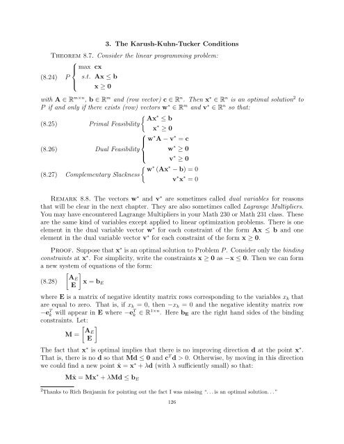
3. The Karush-Kuhn-Tucker Conditions
Theorem 8.7. Consider the linear programming problem:
⎧
⎪⎨
max cx
(8.24) P
⎪⎩
s.t. Ax ≤ b
x ≥ 0
with A ∈ Rm×n , b ∈ Rm and (row vector) c ∈ Rn . Then x∗ ∈ Rn is an optimal solution2 to
P if and only if there exists (row) vectors w∗ ∈ Rm and v∗ ∈ Rn so that:
(8.25)
(8.26)
(8.27)
∗
Ax ≤ b
Primal Feasibility
x ∗ ≥ 0
⎧
⎪⎨
w
Dual Feasibility
⎪⎩
∗ A − v ∗ = c
w ∗ ≥ 0
v ∗ ≥ 0
∗ ∗
w (Ax − b) = 0
Complementary Slackness
v ∗ x ∗ = 0
Remark 8.8. The vectors w ∗ and v ∗ are sometimes called dual variables for reasons
that will be clear in the next chapter. They are also sometimes called Lagrange Multipliers.
You may have encountered Lagrange Multipliers in your Math 230 or Math 231 class. These
are the same kind of variables except applied to linear optimization problems. There is one
element in the dual variable vector w ∗ for each constraint of the form Ax ≤ b and one
element in the dual variable vector v ∗ for each constraint of the form x ≥ 0.
Proof. Suppose that x∗ is an optimal solution to Problem P . Consider only the binding
constraints at x∗ . For simplicity, write the constraints x ≥ 0 as −x ≤ 0. Then we can form
a new system of equations of the form:
AE
(8.28) x = bE
E
where E is a matrix of negative identity matrix rows corresponding to the variables xk that
are equal to zero. That is, if xk = 0, then −xk = 0 and the negative identity matrix row
−e T k will appear in E where −eT k ∈ R1×n . Here bE are the right hand sides of the binding
constraints. Let:
M =
AE
E
The fact that x ∗ is optimal implies that there is no improving direction d at the point x ∗ .
That is, there is no d so that Md ≤ 0 and c T d > 0. Otherwise, by moving in this direction
we could find a new point ˆx = x ∗ + λd (with λ sufficiently small) so that:
Mˆx = Mx ∗ + λMd ≤ bE
2 Thanks to Rich Benjamin for pointing out the fact I was missing “. . . is an optimal solution. . . ”
126