Linear Programming Lecture Notes - Penn State Personal Web Server
Linear Programming Lecture Notes - Penn State Personal Web Server
Linear Programming Lecture Notes - Penn State Personal Web Server
Create successful ePaper yourself
Turn your PDF publications into a flip-book with our unique Google optimized e-Paper software.
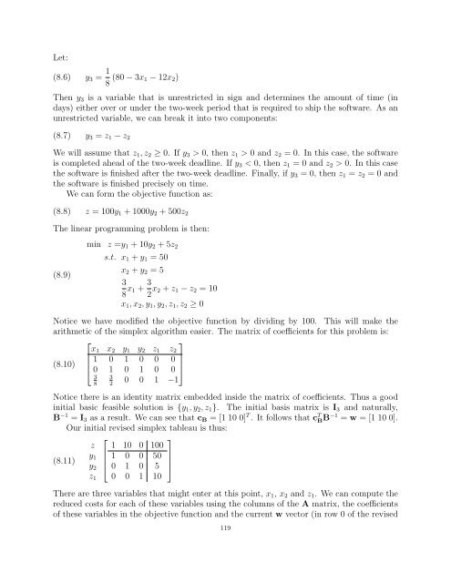
Let:<br />
(8.6) y3 = 1<br />
8 (80 − 3x1 − 12x2)<br />
Then y3 is a variable that is unrestricted in sign and determines the amount of time (in<br />
days) either over or under the two-week period that is required to ship the software. As an<br />
unrestricted variable, we can break it into two components:<br />
(8.7) y3 = z1 − z2<br />
We will assume that z1, z2 ≥ 0. If y3 > 0, then z1 > 0 and z2 = 0. In this case, the software<br />
is completed ahead of the two-week deadline. If y3 < 0, then z1 = 0 and z2 > 0. In this case<br />
the software is finished after the two-week deadline. Finally, if y3 = 0, then z1 = z2 = 0 and<br />
the software is finished precisely on time.<br />
We can form the objective function as:<br />
(8.8) z = 100y1 + 1000y2 + 500z2<br />
The linear programming problem is then:<br />
(8.9)<br />
min z =y1 + 10y2 + 5z2<br />
s.t. x1 + y1 = 50<br />
x2 + y2 = 5<br />
3<br />
8 x1 + 3<br />
2 x2 + z1 − z2 = 10<br />
x1, x2, y1, y2, z1, z2 ≥ 0<br />
Notice we have modified the objective function by dividing by 100. This will make the<br />
arithmetic of the simplex algorithm easier. The matrix of coefficients for this problem is:<br />
⎡<br />
⎤<br />
(8.10)<br />
x1 x2 y1 y2 z1 z2<br />
⎢ 1<br />
⎣ 0<br />
0<br />
1<br />
1<br />
0<br />
0<br />
1<br />
0<br />
0<br />
0 ⎥<br />
0 ⎦<br />
3<br />
8<br />
3<br />
2 0 0 1 −1<br />
Notice there is an identity matrix embedded inside the matrix of coefficients. Thus a good<br />
initial basic feasible solution is {y1, y2, z1}. The initial basis matrix is I3 and naturally,<br />
B −1 = I3 as a result. We can see that cB = [1 10 0] T . It follows that c T B B−1 = w = [1 10 0].<br />
Our initial revised simplex tableau is thus:<br />
z<br />
y1<br />
y2<br />
⎡<br />
1<br />
⎢ 1<br />
⎣ 0<br />
10<br />
0<br />
1<br />
0<br />
0<br />
0<br />
⎤<br />
100<br />
50 ⎥<br />
5 ⎦<br />
0 0 1 10<br />
(8.11)<br />
z1<br />
There are three variables that might enter at this point, x1, x2 and z1. We can compute the<br />
reduced costs for each of these variables using the columns of the A matrix, the coefficients<br />
of these variables in the objective function and the current w vector (in row 0 of the revised<br />
119


