Linear Programming Lecture Notes - Penn State Personal Web Server

CHAPTER 7
Degeneracy and Convergence
In this section, we will consider the problem of degeneracy and prove (at last) that there
is an implementation of the Simplex Algorithm that is guaranteed to converge to an optimal
solution, assuming one exists.
1. Degeneracy Revisited
We’ve already discussed degeneracy. Recall the following theorem from Chapter 5 that
defines degeneracy in terms of the simplex tableau:
Theorem 5.16. Consider Problem P (our linear programming problem). Let B ∈ R m×m be
a basis matrix corresponding to some set of basic variables xB. Let b = B −1 b. If bj = 0 for
some j = 1, . . . , m, then xB = b and xN = 0 is a degenerate extreme point of the feasible
region of Problem P .
We have seen in Example 5.15 that degeneracy can cause us to take extra steps on
our way from an initial basic feasible solution to an optimal solution. When the simplex
algorithm takes extra steps while remaining at the same degenerate extreme point, this is
called stalling. The problem can become much worse; for certain entering variable rules,
the simplex algorithm can become locked in a cycle of pivots each one moving from one
characterization of a degenerate extreme point to the next. The following example from
Beale and illustrated in Chapter 4 of [BJS04] demonstrates the point.
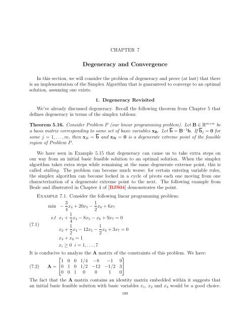
Example 7.1. Consider the following linear programming problem:
min −
(7.1)
3
4 x4 + 20x5 − 1
2 x6 + 6x7
s.t x1 + 1
4 x4 − 8x5 − x6 + 9x7 = 0
x2 + 1
2 x4 − 12x5 − 1
2 x6 + 3x7 = 0
x3 + x6 = 1
xi ≥ 0 i = 1, . . . , 7
It is conducive to analyze the A matrix of the constraints of this problem. We have:
⎡
⎤
1 0 0 1/4 −8 −1 9
(7.2) A = ⎣0 1 0 1/2 −12 −1/2 3⎦
0 0 1 0 0 1 0
The fact that the A matrix contains an identity matrix embedded within it suggests that
an initial basic feasible solution with basic variables x1, x2 and x3 would be a good choice.
109