Linear Programming Lecture Notes - Penn State Personal Web Server

This is not in a form Matlab likes, so we change it by multiplying the constraints by −1
on both sides to obtain:
⎧
min x1 + 1.5x2
⎪⎨ s.t. − 2x1 − 3x2 ≤ −20
⎪⎩
− x1 − 2x2 ≤ −12
x1, x2 ≥ 0
Then we have:
1
c =
1.5
−2 −3
A =
−1 −2
−20
b =
−12
H = r = []
0
l = u = []
0
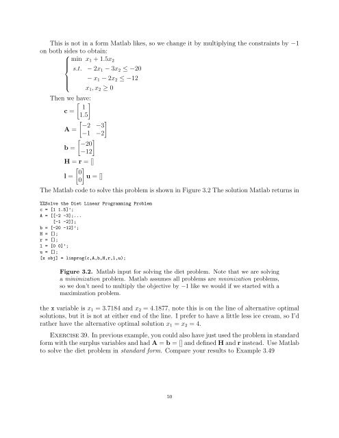
The Matlab code to solve this problem is shown in Figure 3.2 The solution Matlab returns in
%%Solve the Diet Linear Programming Problem
c = [1 1.5]’;
A = [[-2 -3];...
[-1 -2]];
b = [-20 -12]’;
H = [];
r = [];
l = [0 0]’;
u = [];
[x obj] = linprog(c,A,b,H,r,l,u);
Figure 3.2. Matlab input for solving the diet problem. Note that we are solving
a minimization problem. Matlab assumes all problems are mnimization problems,
so we don’t need to multiply the objective by −1 like we would if we started with a
maximization problem.
the x variable is x1 = 3.7184 and x2 = 4.1877, note this is on the line of alternative optimal
solutions, but it is not at either end of the line. I prefer to have a little less ice cream, so I’d
rather have the alternative optimal solution x1 = x2 = 4.
Exercise 39. In previous example, you could also have just used the problem in standard
form with the surplus variables and had A = b = [] and defined H and r instead. Use Matlab
to solve the diet problem in standard form. Compare your results to Example 3.49
50