Linear Programming Lecture Notes - Penn State Personal Web Server

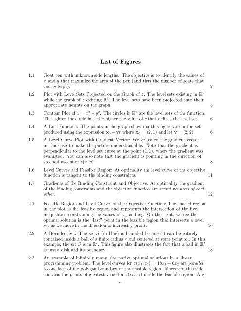
List of Figures
1.1 Goat pen with unknown side lengths. The objective is to identify the values of
x and y that maximize the area of the pen (and thus the number of goats that
can be kept). 2
1.2 Plot with Level Sets Projected on the Graph of z. The level sets existing in R 2
while the graph of z existing R 3 . The level sets have been projected onto their
appropriate heights on the graph. 5
1.3 Contour Plot of z = x 2 + y 2 . The circles in R 2 are the level sets of the function.
The lighter the circle hue, the higher the value of c that defines the level set. 6
1.4 A Line Function: The points in the graph shown in this figure are in the set
produced using the expression x0 + vt where x0 = (2, 1) and let v = (2, 2). 6
1.5 A Level Curve Plot with Gradient Vector: We’ve scaled the gradient vector
in this case to make the picture understandable. Note that the gradient is
perpendicular to the level set curve at the point (1, 1), where the gradient was
evaluated. You can also note that the gradient is pointing in the direction of
steepest ascent of z(x, y). 8
1.6 Level Curves and Feasible Region: At optimality the level curve of the objective
function is tangent to the binding constraints. 11
1.7 Gradients of the Binding Constraint and Objective: At optimality the gradient
of the binding constraints and the objective function are scaled versions of each
other. 12
2.1 Feasible Region and Level Curves of the Objective Function: The shaded region
in the plot is the feasible region and represents the intersection of the five
inequalities constraining the values of x1 and x2. On the right, we see the
optimal solution is the “last” point in the feasible region that intersects a level
set as we move in the direction of increasing profit. 16
2.2 A Bounded Set: The set S (in blue) is bounded because it can be entirely
contained inside a ball of a finite radius r and centered at some point x0. In this
example, the set S is in R 2 . This figure also illustrates the fact that a ball in R 2
is just a disk and its boundary. 18
2.3 An example of infinitely many alternative optimal solutions in a linear
programming problem. The level curves for z(x1, x2) = 18x1 + 6x2 are parallel
to one face of the polygon boundary of the feasible region. Moreover, this side
contains the points of greatest value for z(x1, x2) inside the feasible region. Any
vii