Linear Programming Lecture Notes - Penn State Personal Web Server

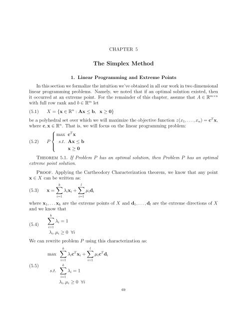
CHAPTER 5
The Simplex Method
1. Linear Programming and Extreme Points
In this section we formalize the intuition we’ve obtained in all our work in two dimensional
linear programming problems. Namely, we noted that if an optimal solution existed, then
it occurred at an extreme point. For the remainder of this chapter, assume that A ∈ R m×n
with full row rank and b ∈ R m let
(5.1) X = {x ∈ R n : Ax ≤ b, x ≥ 0}
be a polyhedral set over which we will maximize the objective function z(x1, . . . , xn) = cT x,
where c, x ∈ Rn . That is, we will focus on the linear programming problem:
⎧
⎪⎨ max c
(5.2) P
⎪⎩
T x
s.t. Ax ≤ b
x ≥ 0
Theorem 5.1. If Problem P has an optimal solution, then Problem P has an optimal
extreme point solution.
Proof. Applying the Cartheodory Characterization theorem, we know that any point
x ∈ X can be written as:
k
l
(5.3) x = λixi +
i=1
i=1
µidi
where x1, . . . xk are the extreme points of X and d1, . . . , dl are the extreme directions of X
and we know that
k
λi = 1
(5.4)
i=1
λi, µi ≥ 0 ∀i
We can rewrite problem P using this characterization as:
(5.5)
max
s.t.
k
i=1
λic T xi +
k
λi = 1
i=1
λi, µi ≥ 0 ∀i
l
i=1
µic T di
69