Linear Programming Lecture Notes - Penn State Personal Web Server

To remove the artificial variables from the basis, let us assume that we can arrange Rows
1 − m of the Phase I simplex tableau as follows:
(6.15)
xB xBa xN xNa RHS
xB Ik 0 R1 R3 b
xBa 0 Im−k R2 R4 0
Column swapping ensures we can do this, if we so desire. Our objective is to replace elements
in xBa (the basic artificial variables) with elements from xN non-basic, non-artificial variables.
Thus, we will attempt to pivot on elements in the matrix R2. Clearly since the Phase I
coefficients of the variables in xN are zero, pivoting in these elements will not negatively
impact the Phase I objective value. Thus, if the element in position (1, 1) is non-zero, then
we can enter the variable xN1 into the basis and remove the variable xBa 1 . This will produce
a new tableau with structure similar to the one given in Equation 6.15 except there will be
k + 1 non-artificial basic variables and m − k − 1 artificial basic variables. Clearly if the
element in position (1, 1) in matrix R2 is zero, then we must move to a different element for
pivoting.
In executing the procedure discussed above, one of two things will occur:
(1) The matrix R2 will be transformed into Im−k or
(2) A point will be reached where there are no longer any variables in xN that can be
entered into the basis because all the elements of R2 are zero.
In the first case, we have removed all the artificial variables from the basis in Phase I
and we can proceed to Phase II with the current basic feasible solution. In the second case,
we will have shown that:
Ik R1
(6.16) A ∼
0 0
This shows that the m − k rows of A are not linearly independent of the first k rows and
thus the matrix A did not have full row rank. When this occurs, we can discard the last
m − k rows of A and simply proceed with the solution given in xB = b, xN = 0. This is a
basic feasible solution to the new matrix A in which we have removed the redundant rows.
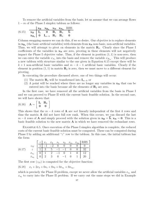
Example 6.5. Once execution of the Phase I simplex algorithm is complete, the reduced
costs of the current basic feasible solution must be computed. These can be computed during
Phase I by adding an additional “z” row to the tableau. In this case, the initial tableau has
the form:
(6.17)
zII
z
xa1
xa2
⎡
⎢
⎣
z x1 x2 s1 s2 xa1 xa2 RHS
1 −1 −2 0 0 0 0 0
1 3 5 −1 −1 0 0 32
0 1 2 −1 0 1 0 12
0 2 3 0 −1 0 1 20
The first row (zII) is computed for the objective function:
(6.18) x1 + 2x2 + 0s1 + 0s2 + 0xa1 + 0xa2,
which is precisely the Phase II problem, except we never allow the artificial variables xa1 and
xa2 to carry into the Phase II problem. If we carry out the same steps we did in Example
97
⎤
⎥
⎦