- Page 1: Linear Programming: Penn State Math
- Page 4 and 5: 8. Caratheodory Characterization Th
- Page 7 and 8: List of Figures 1.1 Goat pen with u
- Page 9 and 10: 4.6 Convex Direction: Clearly every
- Page 11: Preface Stop! Stop right now! This
- Page 14 and 15: x Goat Pen Figure 1.1. Goat pen wit
- Page 16 and 17: We have formulated the general maxi
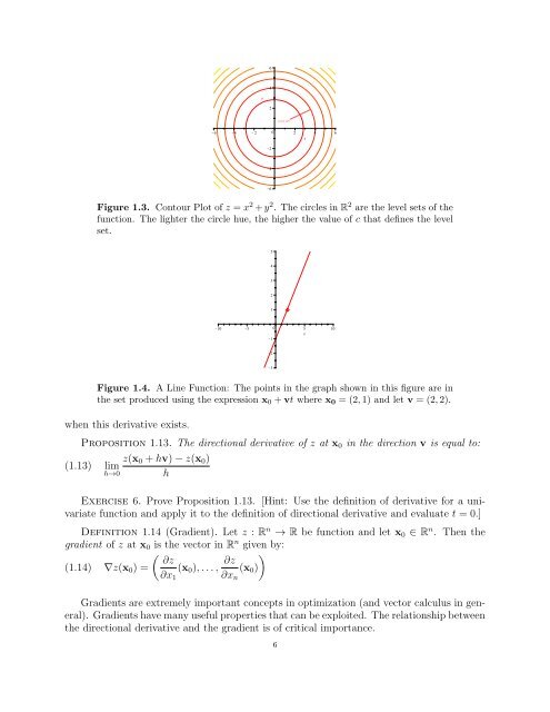
- Page 20 and 21: Figure 1.5. A Level Curve Plot with
- Page 22 and 23: and thus our vector is v = (x1 −
- Page 24 and 25: Figure 1.7. Gradients of the Bindin
- Page 26 and 27: finishing toys and 120 hours per we
- Page 28 and 29: 2. Graphically Solving Linear Progr
- Page 30 and 31: S r x 0 Br( x0) Figure 2.2. A Bound
- Page 32 and 33: S Every point on this line is an al
- Page 34: 6. Problems with Unbounded Feasible
- Page 37: to “prove” your example works.
- Page 40 and 41: Definition 3.6 (Matrix Transpose).
- Page 42 and 43: 3. Matrices and Linear Programming
- Page 44 and 45: Remark 3.16. We can deal with const
- Page 46 and 47: Theorem 3.20. Each elementary row o
- Page 48 and 49: Gauss-Jordan Elimination Computing
- Page 50 and 51: and right hand side vector b = [7,
- Page 52 and 53: Gauss-Jordan elimination to solve t
- Page 54 and 55: which clearly has a solution for al
- Page 56 and 57: which is a contradiction. Case 2: S
- Page 58 and 59: Definition 3.46 (Basic Variables).
- Page 60 and 61: This leads to the following linear
- Page 62 and 63: This is not in a form Matlab likes,
- Page 64 and 65: Example 4.5. Figure 4.1 illustrates
- Page 66 and 67: Figure 4.3. A hyperplane in 3 dimen
- Page 68 and 69:
4. Rays and Directions Recall the d
- Page 70 and 71:
for all λ > 0. This can only be tr
- Page 72 and 73:
Theorem 4.31. Let P ⊆ R n be a po
- Page 74 and 75:
Figure 4.9. A Polyhedral Set: This
- Page 76 and 77:
Figure 4.10. Visualization of the s
- Page 78 and 79:
It is clear that P is bounded. In f
- Page 80 and 81:
x1 x5 x2 x λx2 +(1− λ)x3 x4 x3
- Page 82 and 83:
If there is some i such that c T di
- Page 84 and 85:
Consider now the fact xj = 0 for al
- Page 86 and 87:
Example 5.9. Consider the Toy Maker
- Page 88 and 89:
using this information, we can comp
- Page 90 and 91:
Figure 5.1. The Simplex Algorithm:
- Page 92 and 93:
Using this information, we can see
- Page 94 and 95:
Based on this information, we can c
- Page 96 and 97:
Using the rule you developed in Exe
- Page 98 and 99:
Exercise 52. Consider the diet prob
- Page 100 and 101:
Suppose we choose s4 as the leaving
- Page 103 and 104:
CHAPTER 6 Simplex Initialization In
- Page 105 and 106:
A basic feasible solution for our a
- Page 107 and 108:
variables. This is because we start
- Page 109 and 110:
To remove the artificial variables
- Page 111 and 112:
Remark 6.6. In the case of a minimi
- Page 113 and 114:
Example 6.13. Suppose we solve the
- Page 115 and 116:
That is, s1 = −12 and s2 = −20
- Page 117 and 118:
The complete problem describing McL
- Page 119:
* data section */ data; set DAY :=
- Page 122 and 123:
This leads to a vector of reduced c
- Page 124 and 125:
2.1. Lexicographic Minimum Ratio Te
- Page 126 and 127:
Proof. The initial basis Im yieds a
- Page 128 and 129:
for i = 1, . . . , n. Then we have:
- Page 130 and 131:
Revised Simplex Algorithm (1) Ident
- Page 132 and 133:
simplex tableau). We obtain: z1 −
- Page 134 and 135:
Proof. We can prove Farkas’ Lemma
- Page 136 and 137:
A1· Half-space cy > 0 A2· c Am·
- Page 138 and 139:
3. The Karush-Kuhn-Tucker Condition
- Page 140 and 141:
Remark 8.9. The expressions: ∗ A
- Page 142 and 143:
(x ∗ 1,x ∗ 2) = (16, 72) 3x1 +
- Page 144 and 145:
Since w1, w2 ≥ 0, we know that w
- Page 146 and 147:
Example 8.13. Consider the followin
- Page 148 and 149:
Figure 8.5. This figure illustrates
- Page 150 and 151:
(9.4) Proof. Rewrite Problem D as:
- Page 152 and 153:
This vector will be related to c in
- Page 154 and 155:
3. Strong Duality Lemma 9.7. Proble
- Page 156 and 157:
Likewise beginning with the KKT con
- Page 158 and 159:
egions are polyhedral sets 1 . Cert
- Page 160 and 161:
Figure 9.2. The simplex algorithm b
- Page 162 and 163:
If a selfish profit maximizer wishe
- Page 164 and 165:
Recall the optimal full tableau for
- Page 166 and 167:
For the sake of space, we will prov
- Page 168 and 169:
We can choose either s1 or s2 as a