Linear Programming Lecture Notes - Penn State Personal Web Server

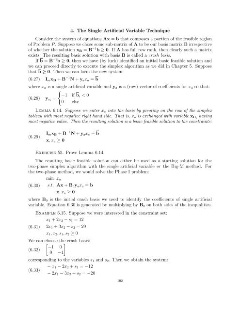
4. The Single Artificial Variable Technique
Consider the system of equations Ax = b that composes a portion of the feasible region
of Problem P . Suppose we chose some sub-matrix of A to be our basis matrix B irrespective
of whether the solution xB = B −1 b ≥ 0. If A has full row rank, then clearly such a matrix
exists. The resulting basic solution with basis B is called a crash basis.
If b = B −1 b ≥ 0, then we have (by luck) identified an initial basic feasible solution and
we can proceed directly to execute the simplex algorithm as we did in Chapter 5. Suppose
that b ≥ 0. Then we can form the new system:
(6.27) ImxB + B −1 N + yaxa = b
where xa is a single artificial variable and ya is a (row) vector of coefficients for xa so that:
(6.28) yai =
−1 if bi < 0
0 else
Lemma 6.14. Suppose we enter xa into the basis by pivoting on the row of the simplex
tableau with most negative right hand side. That is, xa is exchanged with variable xBj having
most negative value. Then the resulting solution is a basic feasible solution to the constraints:
(6.29)
ImxB + B −1 N + yaxa = b
x, xa ≥ 0
Exercise 55. Prove Lemma 6.14.
The resulting basic feasible solution can either be used as a starting solution for the
two-phase simplex algorithm with the single artificial variable or the Big-M method. For
the two-phase method, we would solve the Phase I problem:
(6.30)
min xa
s.t. Ax + B0yaxa = b
x, xa ≥ 0
where B0 is the initial crash basis we used to identify the coefficients of single artificial
variable. Equation 6.30 is generated by multiplying by B0 on both sides of the inequalities.
(6.31)
Example 6.15. Suppose we were interested in the constraint set:
x1 + 2x2 − s1 = 12
2x1 + 3x2 − s2 = 20
x1, x2, s1, s2 ≥ 0
We can choose the crash basis:
−1 0
(6.32)
0 −1
corresponding to the variables s1 and s2. Then we obtain the system:
(6.33)
− x1 − 2x2 + s1 = −12
− 2x1 − 3x2 + s2 = −20
102