Linear Programming Lecture Notes - Penn State Personal Web Server

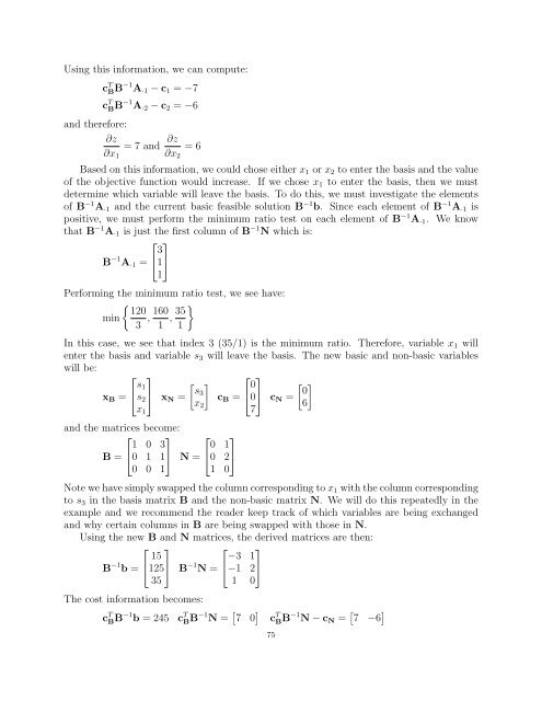
Using this information, we can compute:
c T BB −1 A·1 − c1 = −7
c T BB −1 A·2 − c2 = −6
and therefore:
∂z
∂x1
= 7 and ∂z
∂x2
= 6
Based on this information, we could chose either x1 or x2 to enter the basis and the value
of the objective function would increase. If we chose x1 to enter the basis, then we must
determine which variable will leave the basis. To do this, we must investigate the elements
of B−1A·1 and the current basic feasible solution B−1b. Since each element of B−1A·1 is
positive, we must perform the minimum ratio test on each element of B−1A·1. We know
that B−1A·1 is just the first column of B−1N which is:
B −1 A·1 =
⎡
⎣ 3
⎤
1⎦
1
Performing the minimum ratio test, we see have:
120 160 35
min , ,
3 1 1
In this case, we see that index 3 (35/1) is the minimum ratio. Therefore, variable x1 will
enter the basis and variable s3 will leave the basis. The new basic and non-basic variables
will be:
⎡
xB = ⎣ s1
s2
x1
⎤
⎦ xN =
s3
x2
cB =
and the matrices become:
⎡ ⎤ ⎡
1 0 3 0
B = ⎣0 1 1⎦
N = ⎣0 ⎤
1
2⎦
0 0 1 1 0
⎡
⎣ 0
⎤
0⎦
cN =
7
Note we have simply swapped the column corresponding to x1 with the column corresponding
to s3 in the basis matrix B and the non-basic matrix N. We will do this repeatedly in the
example and we recommend the reader keep track of which variables are being exchanged
and why certain columns in B are being swapped with those in N.
0
6
Using the new B and N matrices, the derived matrices are then:
B −1 ⎡
b = ⎣ 15
⎤
125⎦
B
35
−1 ⎡
−3
N = ⎣−1 ⎤
1
2⎦
1 0
The cost information becomes:
c T BB −1 b = 245 c T BB −1 N = 7 0 c T BB −1 N − cN = 7 −6
75