Linear Programming Lecture Notes - Penn State Personal Web Server

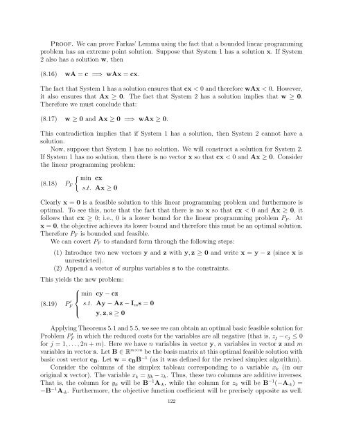
Proof. We can prove Farkas’ Lemma using the fact that a bounded linear programming
problem has an extreme point solution. Suppose that System 1 has a solution x. If System
2 also has a solution w, then
(8.16) wA = c =⇒ wAx = cx.
The fact that System 1 has a solution ensures that cx < 0 and therefore wAx < 0. However,
it also ensures that Ax ≥ 0. The fact that System 2 has a solution implies that w ≥ 0.
Therefore we must conclude that:
(8.17) w ≥ 0 and Ax ≥ 0 =⇒ wAx ≥ 0.
This contradiction implies that if System 1 has a solution, then System 2 cannot have a
solution.
Now, suppose that System 1 has no solution. We will construct a solution for System 2.
If System 1 has no solution, then there is no vector x so that cx < 0 and Ax ≥ 0. Consider
the linear programming problem:
min cx
(8.18) PF
s.t. Ax ≥ 0
Clearly x = 0 is a feasible solution to this linear programming problem and furthermore is
optimal. To see this, note that the fact that there is no x so that cx < 0 and Ax ≥ 0, it
follows that cx ≥ 0; i.e., 0 is a lower bound for the linear programming problem PF . At
x = 0, the objective achieves its lower bound and therefore this must be an optimal solution.
Therefore PF is bounded and feasible.
We can covert PF to standard form through the following steps:
(1) Introduce two new vectors y and z with y, z ≥ 0 and write x = y − z (since x is
unrestricted).
(2) Append a vector of surplus variables s to the constraints.
This yields the new problem:
(8.19) P ′ ⎧
⎪⎨
min cy − cz
s.t. Ay − Az − Ims = 0
F
⎪⎩
y, z, s ≥ 0
Applying Theorems 5.1 and 5.5, we see we can obtain an optimal basic feasible solution for
Problem P ′ F in which the reduced costs for the variables are all negative (that is, zj − cj ≤ 0
for j = 1, . . . , 2n + m). Here we have n variables in vector y, n variables in vector z and m
variables in vector s. Let B ∈ R m×m be the basis matrix at this optimal feasible solution with
basic cost vector cB. Let w = cBB −1 (as it was defined for the revised simplex algorithm).
Consider the columns of the simplex tableau corresponding to a variable xk (in our
original x vector). The variable xk = yk − zk. Thus, these two columns are additive inverses.
That is, the column for yk will be B −1 A·k, while the column for zk will be B −1 (−A·k) =
−B −1 A·k. Furthermore, the objective function coefficient will be precisely opposite as well.
122