
Create successful ePaper yourself
Turn your PDF publications into a flip-book with our unique Google optimized e-Paper software.
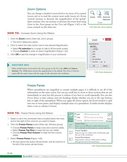
Zoom Options<br />
You can change a window’s zoom level to see more of its content<br />
(zoom out) or to read the content more easily (zoom in). Zoom<br />
controls increase or decrease the magnification of the spreadsheet<br />
contents. You can increase or decrease the zoom level using<br />
Zoom in the Zoom group on the View tab (Figure 1-63) or the<br />
zoom controls on the Status bar.<br />
1-63 View tab, Zoom options<br />
HOW TO: Increase Zoom Using the Ribbon<br />
1. Click the Zoom button [View tab, Zoom group].<br />
• The Zoom dialog box opens.<br />
2. Click to select the radio button next to the desired Magnification.<br />
• Select Fit selection for a range of cells to fill the entire screen.<br />
• Choose Custom to enter an exact magnification (Figure 1-64).<br />
3. Click OK to see the change in magnification in your workbook.<br />
ANOTHER WAY<br />
Other useful buttons are located in the Zoom group on the View tab: 100% and Zoom to<br />
Selection. The 100% option returns the magnification to the default. The Zoom to Selection<br />
option fills the entire screen with the range of cells selected in the worksheet.<br />
1-64 Zoom dialog box<br />
Freeze Panes<br />
When spreadsheets are magnified or contain multiple pages, it is difficult to see all of the<br />
information on the same screen. You can use scroll bars to move to those sections that are not<br />
immediately in view, but this process is tedious if you have to scroll repeatedly. You can also<br />
Freeze Panes so that column and row headings display whether you are at the top, bottom,<br />
left, or right of the spreadsheet. When you apply the freeze option, the <strong>Excel</strong> window is split<br />
into one or more panes, and displays multiple areas of a spreadsheet. A darker border displays<br />
when a row or column is frozen.<br />
HOW TO: Freeze Panes Using the Ribbon<br />
1. Select a cell in the worksheet that is located below the rows<br />
and to the right of the columns you want to freeze.<br />
2. Click the Freeze Panes button [View tab, Window group].<br />
• Choose Freeze Panes to keep rows and columns visible.<br />
• Select Freeze Top Row to keep the top row visible.<br />
• Choose Freeze First Column to keep the first column<br />
visible.<br />
3. Select Freeze Panes (Figure 1-65).<br />
• All rows above the active cell are frozen, and all columns to<br />
the left of the active cell are frozen.<br />
1-65 Freeze Panes button<br />
E1-38<br />
<strong>Excel</strong> 2013 <strong>Chapter</strong> 1 Creating and Editing Workbooks