Direct Power and Torque Control of AC/DC/AC Converter-Fed ...

3. Vector Control Methods of AC/DC/AC Converter-Fed IM Drives – A Review
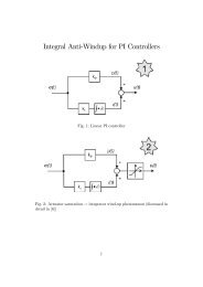
The step answer of the system with implemented decoupling in power control loop is
presented in Fig. 3. 26 (reference step at 0.4 [ s]
[] s
t = 0.41 ).
t = and disturbance step at
500.0
a)
450.0
400.0
350.0
300.0
250.0
200.0
150.0
100.0
50.0
0.0
-50.0
-100.0
-150.0
500.0
b)
450.0
400.0
350.0
300.0
250.0
200.0
150.0
100.0
50.0
0.0
-50.0
-100.0
-150.0
0.396 0.398 0.4 0.402 0.404 0.406 0.408 0.41 0.412
0.396 0.398 0.4 0.402 0.404 0.406 0.408 0.41 0.412
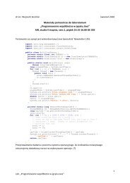
Fig. 3. 26. Active power tracking performance (simulated in Saber) with decoupling;
without prefilter, b) with prefilter
From the top: command and estimated active power, command and estimated reactive power
The response is closer to ideal one obtained in Matlab. However, there is still
difference. It is caused by not fully decoupled signals and effect of sampling time T
S
of discrete control system.
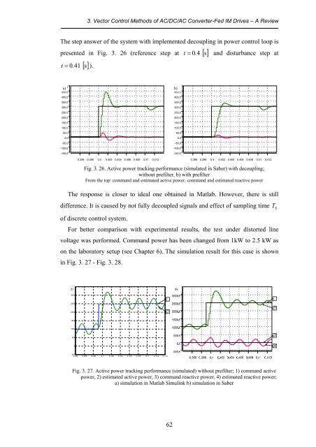
For better comparison with experimental results, the test under distorted line
voltage was performed. Command power has been changed from 1kW to 2.5 kW as
on the laboratory setup (see Chapter 6). The simulation result for this case is shown
in Fig. 3. 27 - Fig. 3. 28.
3500
3000
2500
2000
1500
1000
500
0
-500
0.094 0.096 0.098 0.1 0.102 0.104 0.106 0.108 0.11 0.112 0.114
Fig. 3. 27. Active power tracking performance (simulated) without prefilter; 1) command active
power, 2) estimated active power, 3) command reactive power, 4) estimated reactive power;
a) simulation in Matlab Simulink b) simulation in Saber
62