The Palestinian Economy. Theoretical and Practical Challenges
The Palestinian Economy. Theoretical and Practical Challenges
The Palestinian Economy. Theoretical and Practical Challenges

Create successful ePaper yourself
Turn your PDF publications into a flip-book with our unique Google optimized e-Paper software.
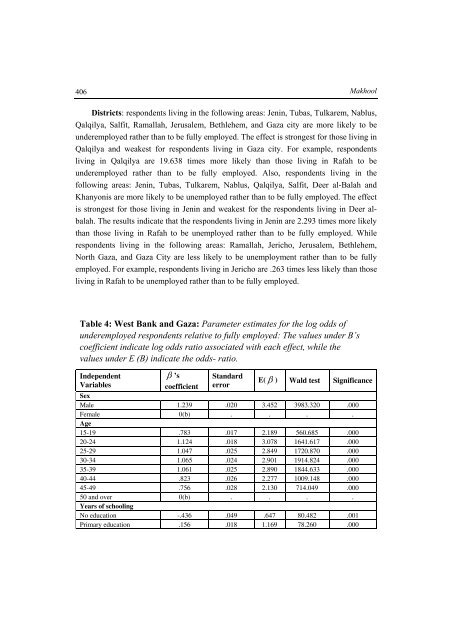
406<br />
Makhool<br />
Districts: respondents living in the following areas: Jenin, Tubas, Tulkarem, Nablus,<br />
Qalqilya, Salfit, Ramallah, Jerusalem, Bethlehem, <strong>and</strong> Gaza city are more likely to be<br />
underemployed rather than to be fully employed. <strong>The</strong> effect is strongest for those living in<br />
Qalqilya <strong>and</strong> weakest for respondents living in Gaza city. For example, respondents<br />
living in Qalqilya are 19.638 times more likely than those living in Rafah to be<br />
underemployed rather than to be fully employed. Also, respondents living in the<br />
following areas: Jenin, Tubas, Tulkarem, Nablus, Qalqilya, Salfit, Deer al-Balah <strong>and</strong><br />
Khanyonis are more likely to be unemployed rather than to be fully employed. <strong>The</strong> effect<br />
is strongest for those living in Jenin <strong>and</strong> weakest for the respondents living in Deer albalah.<br />
<strong>The</strong> results indicate that the respondents living in Jenin are 2.293 times more likely<br />
than those living in Rafah to be unemployed rather than to be fully employed. While<br />
respondents living in the following areas: Ramallah, Jericho, Jerusalem, Bethlehem,<br />
North Gaza, <strong>and</strong> Gaza City are less likely to be unemployment rather than to be fully<br />
employed. For example, respondents living in Jericho are .263 times less likely than those<br />
living in Rafah to be unemployed rather than to be fully employed.<br />
Table 4: West Bank <strong>and</strong> Gaza: Parameter estimates for the log odds of<br />
underemployed respondents relative to fully employed: <strong>The</strong> values under B’s<br />
coefficient indicate log odds ratio associated with each effect, while the<br />
values under E (B) indicate the odds- ratio.<br />
Independent<br />
Variables<br />
’s<br />
coefficient<br />
St<strong>and</strong>ard<br />
error<br />
E( ) Wald test Significance<br />
Sex<br />
Male 1.239 .020 3.452 3983.320 .000<br />
Female 0(b) . . . .<br />
Age<br />
15-19 .783 .017 2.189 560.685 .000<br />
20-24 1.124 .018 3.078 1641.617 .000<br />
25-29 1.047 .025 2.849 1720.870 .000<br />
30-34 1.065 .024 2.901 1914.824 .000<br />
35-39 1.061 .025 2.890 1844.633 .000<br />
40-44 .823 .026 2.277 1009.148 .000<br />
45-49 .756 .028 2.130 714.049 .000<br />
50 <strong>and</strong> over 0(b) . . . .<br />
Years of schooling<br />
No education -.436 .049 .647 80.482 .001<br />
Primary education .156 .018 1.169 78.260 .000