Market Economics | Interest Rate Strategy - BNP PARIBAS ...

The sensitivity of the spread curve to 1y OIS/Bor is
once again 40%, which provides some level of
comfort with this hedge ratio.
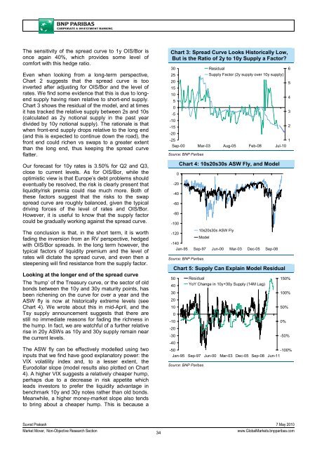
Even when looking from a long-term perspective,
Chart 2 suggests that the spread curve is too
inverted after adjusting for OIS/Bor and the level of
rates. We find some evidence that this is due to longend
supply having risen relative to short-end supply.
Chart 3 shows the residual of the model, and at times
it has tracked the relative supply between 2s and 10s
(calculated as 2y notional supply in the past year
divided by 10y notional supply). The rationale is that
when front-end supply drops relative to the long end
(and this is expected to continue down the road), the
front end could richen vs swaps to a greater extent
than the long end, thus keeping the spread curve
flatter.
Our forecast for 10y rates is 3.50% for Q2 and Q3,
close to current levels. As for OIS/Bor, while the
optimistic view is that Europe’s debt problems should
eventually be resolved, the risk is clearly present that
liquidity/risk premia could rise much more. Both of
these factors suggest that the risks to the swap
spread curve are roughly balanced, given the typical
driving forces of the level of rates and OIS/Bor.
However, it is useful to know that the supply factor
could be gradually working against the spread curve.
The conclusion is that, in the short term, it is worth
fading the inversion from an RV perspective, hedged
with OIS/Bor spreads. In the long term however, the
typical factors of liquidity premium and the level of
rates will dictate the spread curve, and even then a
steepening will find resistance from the supply factor.
Looking at the longer end of the spread curve
The ‘hump’ of the Treasury curve, or the sector of old
bonds between the 10y and 30y maturity points, has
been richening on the curve for over a year and the
ASW fly is now at historically extreme levels (see
Chart 4). We wrote about this in mid-April, and the
Tsy supply announcement suggests that there are
still no immediate reasons for fading the richness in
the hump. In fact, we are watchful of a further relative
rise in 20y ASWs as 10y and 30y supply remain near
the current levels.
The ASW fly can be effectively modelled using two
inputs that we find have good explanatory power: the
VIX volatility index and, to a lesser extent, the
Eurodollar slope (model results also plotted on Chart
4). A higher VIX suggests a relatively cheaper hump,
perhaps due to a decrease in risk appetite which
leads investors to prefer the liquidity advantage in
benchmark 10y and 30y notes rather than old bonds.
Meanwhile, a higher money-market slope also tends
to bring about a cheaper hump. This is because a
Chart 3: Spread Curve Looks Historically Low,
But is the Ratio of 2y to 10y Supply a Factor?
30
25
Residual
Supply Factor (2y supply over 10y supply)
6
20
5
15
10
4
5
0
-5
3
-10
-15
2
-20
-25
1
Sep-00 Mar-03 Aug-05 Feb-08 Jul-10
Source: BNP Paribas
0
-20
-40
-60
-80
-100
-120
Chart 4: 10s20s30s ASW Fly, and Model
10s20s30s ASW Fly
Model
-140
Jan-95 Sep-97 Jun-00 Mar-03 Dec-05 Sep-08
Source: BNP Paribas
50
40
30
20
10
-10
-20
-30
-40
Chart 5: Supply Can Explain Model Residual
0
-50%
-50
-100%
Jan-95 Sep-97 Jun-00 Mar-03 Dec-05 Sep-08 Jun-11
Source: BNP Paribas
Residual
YoY Change in 10y+30y Supply (14M Lag)
150%
100%
50%
0%
Suvrat Prakash 7 May 2010
Market Mover, Non-Objective Research Section
34
www.GlobalMarkets.bnpparibas.com