DIFFERENTIAL GEOMETRY: A First Course in Curves and Surfaces

More documents

Recommendations

Info

100 Chapter 3. Surfaces: Further Topicsb. Compute ω 12 and dω 12 and verify that K = −1.9. Use moving frames to redoa. Exercise 3.1.9b. Exercise 3.1.1010. a. Use moving frames to reprove the result of Exercise 2.3.13.b. Suppose there are two families of geodesics in M making a constant angle θ. Prove ordisprove: M is flat.11. Recall that locally any 1-form φ with dφ =0can be written in the form φ = df for somefunction f.a. Prove that if a surface M is flat, then locally we can find a moving frame e 1 , e 2 on M sothat ω 12 =0. (Hint: Start with an arbitrary moving frame.)b. Deduce that if M is flat, locally we can find a parametrization x of M with E = G =1and F =0. (That is, locally M is isometric to a plane.)12. (The Bäcklund transform) Suppose M and M are two surfaces in R 3 and f : M → M is asmooth bijective function with the properties that(i) the line from P to f(P )istangent to M at P and tangent to M at f(P );(ii) the distance between P and f(P )isaconstant r, independent of P ;(iii) the angle between n(P ) and n(f(P )) is a constant θ, independent of P .Prove that both M and M have constant curvature K = −(sin 2 θ)/r 2 . (Hints: Write P = f(P ),and let e 1 , e 2 , e 3 (resp. e 1 , e 2 , e 3 )bemoving frames at P (resp. P ) with e 1 = e 1 in the directionof −→P P . Letting x and x = f ◦x be local parametrizations, we have x = x + re 1 . Differentiatethis equation and deduce that ω 12 = cot θω 13 − 1 r ω 2.)4. Calculus of Variations and Surfaces of Constant Mean CurvatureEvery student of calculus is familiar with the necessary condition for a differentiable functionf : R n → R to have a local extreme point (minimum or maximum) at P :Wemust have ∇f(P )=0.Phrased slightly differently, for every vector V, the directional derivativef(P + εV) − f(P )D V f(P )=limε→0 εshould vanish. Moreover, if we are given a constraint set M = {x ∈ R n : g 1 (x) =0,g 2 (x) =0,...,g k (x) =0}, the method of Lagrange multipliers tells us that at a constrained extreme pointP we must havek∑∇f(P )= λ i ∇g i (P )i=1for some scalars λ 1 ,...,λ k . (There is also a nondegeneracy hypothesis here that ∇g 1 (P ),...,∇g k (P )be linearly independent.)Suppose we are given a regular parametrized surface x: U → R 3 and want to find—without thebenefit of the analysis of Section 4 of Chapter 2—a geodesic from P = x(u 0 ,v 0 )toQ = x(u 1 ,v 1 ).
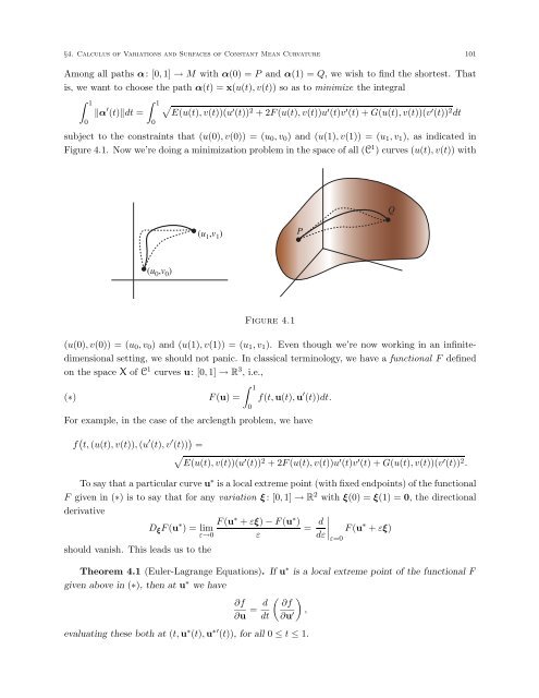
§4. Calculus of Variations and Surfaces of Constant Mean Curvature 101Among all paths α: [0, 1] → M with α(0) = P and α(1) = Q, wewish to find the shortest. Thatis, we want to choose the path α(t) =x(u(t),v(t)) so as to minimize the integral∫ 10‖α ′ (t)‖dt =∫ 10√E(u(t),v(t))(u ′ (t)) 2 +2F (u(t),v(t))u ′ (t)v ′ (t)+G(u(t),v(t))(v ′ (t)) 2 dtsubject to the constraints that (u(0),v(0)) = (u 0 ,v 0 ) and (u(1),v(1)) = (u 1 ,v 1 ), as indicated inFigure 4.1. Now we’re doing a minimization problem in the space of all (C 1 ) curves (u(t),v(t)) with(u 1 ,v 1 ) PQ(u 0 ,v 0 )Figure 4.1(u(0),v(0)) = (u 0 ,v 0 ) and (u(1),v(1)) = (u 1 ,v 1 ). Even though we’re now working in an infinitedimensionalsetting, we should not panic. In classical terminology, we have a functional F definedon the space X of C 1 curves u: [0, 1] → R 3 , i.e.,(∗)F (u) =∫ 10f(t, u(t), u ′ (t))dt.For example, in the case of the arclength problem, we havef ( t, (u(t),v(t)), (u ′ (t),v ′ (t)) ) =√E(u(t),v(t))(u ′ (t)) 2 +2F (u(t),v(t))u ′ (t)v ′ (t)+G(u(t),v(t))(v ′ (t)) 2 .To say that a particular curve u ∗ is a local extreme point (with fixed endpoints) of the functionalF given in (∗) istosay that for any variation ξ :[0, 1] → R 2 with ξ(0) = ξ(1) = 0, the directionalderivativeshould vanish. This leads us to theD ξ F (u ∗ )=limε→0F (u ∗ + εξ) − F (u ∗ )ε= d dε∣ F (u ∗ + εξ)ε=0Theorem 4.1 (Euler-Lagrange Equations). If u ∗ is a local extreme point of the functional Fgiven above in (∗), then at u ∗ we have∂f∂u = d ( ) ∂fdt ∂u ′ ,evaluating these both at (t, u ∗ (t), u ∗′ (t)), for all 0 ≤ t ≤ 1.
Page 1:
DIFFERENTIALGEOMETRY:A First Course
Page 6 and 7:
4 Chapter 1. Curves2πb2πaFigure 1
Page 8 and 9:
6 Chapter 1. CurvesAlternatively, s
Page 10 and 11:
8 Chapter 1. CurvesAn important obs
Page 12 and 13:
10 Chapter 1. Curvesof the road, st
Page 14 and 15:
12 Chapter 1. CurvesSummarizing,κ(
Page 16 and 17:
14 Chapter 1. Curvescurvature κ. I
Page 18 and 19:
16 Chapter 1. CurvesFigure 2.2Conve
Page 20 and 21:
18 Chapter 1. Curvesalso Exercise 2
Page 22 and 23:
20 Chapter 1. Curvesto the curve β
Page 24 and 25:
22 Chapter 1. Curvesthe osculating
Page 26 and 27:
24 Chapter 1. CurvesWe turn now to
Page 28 and 29:
26 Chapter 1. Curvesintersect C eit
Page 30 and 31:
28 Chapter 1. Curvesh(s,t)α(t)α(s
Page 32 and 33:
30 Chapter 1. Curvesy( x(s) ,y(s))
Page 34 and 35:
32 Chapter 1. Curvesɛ2ɛ 1ɛ 3CFig
Page 36 and 37:
CHAPTER 2Surfaces: Local Theory1. P
Page 38 and 39:
36 Chapter 2. Surfaces: Local Theor
Page 40 and 41:
Page 42 and 43:
Page 44 and 45:
Page 46 and 47:
Page 48 and 49:
Page 50 and 51:
Page 52 and 53: 50 Chapter 2. Surfaces: Local Theor
Page 78 and 79: 76 Chapter 3. Surfaces: Further Top
Page 104 and 105: 102 Chapter 3. Surfaces: Further To
Page 110 and 111: 108 Appendix. Review of Linear Alge
Page 116 and 117: ANSWERS TO SELECTED EXERCISES1.1.1
Page 118 and 119: 116 SELECTED ANSWERS2.4.8 Only circ
Page 120: 118 INDEXisometry, 107K, 48k-point
show all

DIFFERENTIAL GEOMETRY: A First Course in Curves and Surfaces

You also want an ePaper? Increase the reach of your titles

Delete template?

Save as template?