DIFFERENTIAL GEOMETRY: A First Course in Curves and Surfaces

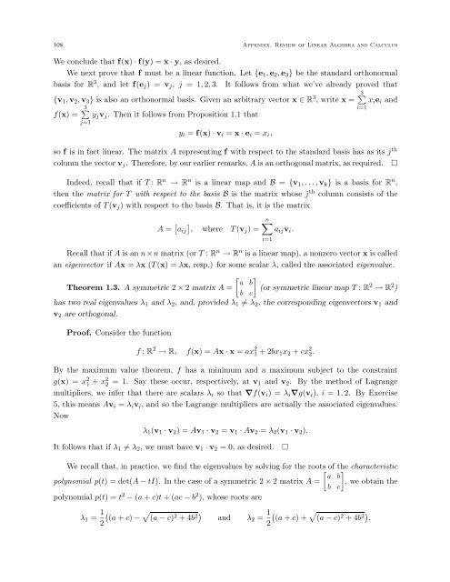
108 Appendix. Review of Linear Algebra and CalculusWe conclude that f(x) · f(y) =x · y, asdesired.We next prove that f must be a linear function. Let {e 1 , e 2 , e 3 } be the standard orthonormalbasis for R 3 , and let f(e j ) = v j , j = 1, 2, 3. It follows from what we’ve already proved that{v 1 , v 2 , v 3 } is also an orthonormal basis. Given an arbitrary vector x ∈ R 3 ∑, write x = 3 x i e i andf(x) =3 ∑j=1y j v j . Then it follows from Proposition 1.1 thaty i = f(x) · v i = x · e i = x i ,so f is in fact linear. The matrix A representing f with respect to the standard basis has as its j thcolumn the vector v j . Therefore, by our earlier remarks, A is an orthogonal matrix, as required. □Indeed, recall that if T : R n → R n is a linear map and B = {v 1 ,...,v k } is a basis for R n ,then the matrix for T with respect to the basis B is the matrix whose j th column consists of thecoefficients of T (v j ) with respect to the basis B. That is, it is the matrixi=1A = [ a ij], where T (vj )=n∑a ij v i .i=1Recall that if A is an n×n matrix (or T : R n → R n is a linear map), a nonzero vector x is calledan eigenvector if Ax = λx (T (x) =λx, resp.) for some scalar λ, called the associated eigenvalue.[ ] a bTheorem 1.3. A symmetric 2 × 2 matrix A = (or symmetric linear map T : R 2 → R 2 )b chas two real eigenvalues λ 1 and λ 2 , and, provided λ 1 ≠ λ 2 , the corresponding eigenvectors v 1 andv 2 are orthogonal.Proof. Consider the functionf : R 2 → R, f(x) =Ax · x = ax 2 1 +2bx 1 x 2 + cx 2 2.By the maximum value theorem, f has a minimum and a maximum subject to the constraintg(x) =x 2 1 + x2 2 =1. Say these occur, respectively, at v 1 and v 2 . By the method of Lagrangemultipliers, we infer that there are scalars λ i so that ∇f(v i )=λ i ∇g(v i ), i =1, 2. By Exercise5, this means Av i = λ i v i , and so the Lagrange multipliers are actually the associated eigenvalues.Nowλ 1 (v 1 · v 2 )=Av 1 · v 2 = v 1 · Av 2 = λ 2 (v 1 · v 2 ).It follows that if λ 1 ≠ λ 2 ,wemust have v 1 · v 2 =0,asdesired.□We recall that, in practice, we find the eigenvalues by solving for the roots[of the]characteristica bpolynomial p(t) =det(A − tI). In the case of a symmetric 2 × 2 matrix A = ,weobtain theb cpolynomial p(t) =t 2 − (a + c)t +(ac − b 2 ), whose roots areλ 1 = 1 ( √(a + c) − (a − c)22 +4b 2) and λ 2 = 1 2((a + c)+√(a − c) 2 +4b 2) .