DIFFERENTIAL GEOMETRY: A First Course in Curves and Surfaces

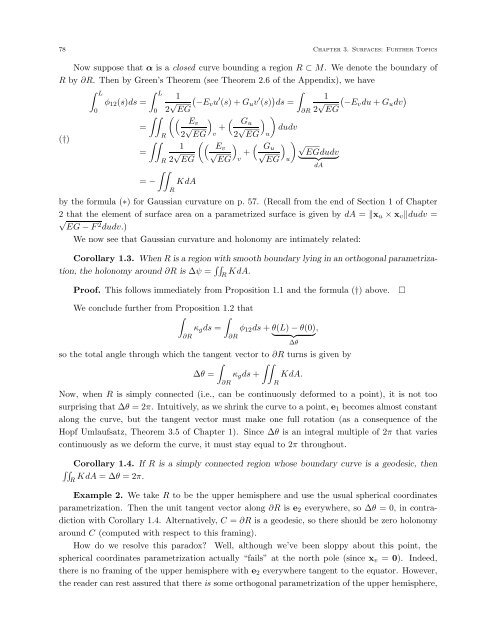
78 Chapter 3. Surfaces: Further TopicsNow suppose that α is a closed curve bounding a region R ⊂ M. Wedenote the boundary ofR by ∂R. Then by Green’s Theorem (see Theorem 2.6 of the Appendix), we have∫ L∫ L1φ 12 (s)ds =00 2 √ (−Ev u ′ (s)+G u v ′ (s) ) ∫1ds =EG∂R 2 √ (−Ev du + G u dv )EG∫∫ ( ( Ev) (=R 2 √ EG+ Gu) )v 2 √ dudvEG u(†)∫∫ (1 (=R 2 √ Ev) (√EG+ Gu) ) √EGdudv√EG v EG u } {{ }dA∫∫= − KdARby the formula (∗) for Gaussian curvature on p. 57. (Recall from the end of Section 1 of Chapter2 that the element of surface area on a parametrized surface is given by dA = ‖x u × x v ‖dudv =√EG − F 2 dudv.)We now see that Gaussian curvature and holonomy are intimately related:Corollary 1.3. When R is a region with smooth boundary lying in an orthogonal parametrization,the holonomy around ∂R is ∆ψ = ∫∫ R KdA.Proof. This follows immediately from Proposition 1.1 and the formula (†) above.□We conclude further from Proposition 1.2 that∫ ∫κ g ds = φ 12 ds + θ(L) − θ(0) ,∂R∂R } {{ }∆θso the total angle through which the tangent vector to ∂R turns is given by∫ ∫∫∆θ = κ g ds + KdA.∂RRNow, when R is simply connected (i.e., can be continuously deformed to a point), it is not toosurprising that ∆θ =2π. Intuitively, as we shrink the curve to a point, e 1 becomes almost constantalong the curve, but the tangent vector must make one full rotation (as a consequence of theHopf Umlaufsatz, Theorem 3.5 of Chapter 1). Since ∆θ is an integral multiple of 2π that variescontinuously as we deform the curve, it must stay equal to 2π throughout.Corollary 1.4. If R is a simply connected region whose boundary curve is a geodesic, then∫∫KdA =∆θ =2π.RExample 2. We take R to be the upper hemisphere and use the usual spherical coordinatesparametrization. Then the unit tangent vector along ∂R is e 2 everywhere, so ∆θ =0,incontradictionwith Corollary 1.4. Alternatively, C = ∂R is a geodesic, so there should be zero holonomyaround C (computed with respect to this framing).How do we resolve this paradox? Well, although we’ve been sloppy about this point, thespherical coordinates parametrization actually “fails” at the north pole (since x v = 0). Indeed,there is no framing of the upper hemisphere with e 2 everywhere tangent to the equator. However,the reader can rest assured that there is some orthogonal parametrization of the upper hemisphere,