DIFFERENTIAL GEOMETRY: A First Course in Curves and Surfaces

More documents

Recommendations

Info

54 Chapter 2. Surfaces: Local Theoryc. Suppose M is represented locally near P as in Exercise 20. Show that for small positivevalues of c, the intersection of M with the plane z = c “looks like” the Dupin indicatrix.How can you make this statement more precise?22. Suppose the surface M is given near P as a level surface of a smooth function f : R 3 → R with∇f(P ) ≠0.Aline L ⊂ R 3 is said to have (at least) k-point contact with M at P if, given anylinear parametrization α of L with α(0) = P , the function f = f ◦α vanishes to order k − 1,i.e., f(0) = f ′ (0) = ···= f (k−1) (0) = 0. (Such a line is to be visualized as the limit of lines thatintersect M at P and at k − 1 other points that approach P .)a. Show that L has 2-point contact with M at P if and only if L is tangent to M at P , i.e.,L ⊂ T P M.b. Show that L has 3-point contact with M at P if and only if L is an asymptotic directionat P . (Hint: It may be helpful to follow the setup of Exercise 20.)c. (Challenge) What does it mean for L to have 4-point contact with M at P ?3. The Codazzi and Gauss Equations and the Fundamental Theorem of SurfaceTheoryWe now wish to proceed towards a deeper understanding of Gaussian curvature. We have tothis point considered only the normal components of the second derivatives x uu , x uv , and x vv .Nowlet’s consider them in toto. Since {x u , x v , n} gives a basis for R 3 , there are functions Γuu, u Γuu,vΓuv u =Γvu, u Γuv v =Γvu, v Γvv, u and Γvv v so that(†)x uu =Γ u uux u +Γ v uux v + lnx uv =Γ u uvx u +Γ v uvx v + mnx vv =Γ uvvx u +Γ vvvx v + nn.(Note that x uv = x vu dictates the symmetries Γ uv • =Γ vu.) • The functions Γ •• • are called Christoffelsymbols.Example 1. Let’s compute the Christoffel symbols for the usual parametrization of the sphere.By straightforward calculation we obtainx u = (cos u cos v, cos u sin v, − sin u)x v =(− sin u sin v, sin u cos v, 0)x uu =(− sin u cos v, − sin u sin v, − cos u) =−x(u, v)x uv =(− cos u sin v, cos u cos v, 0)x vv =(− sin u cos v, − sin u sin v, 0) = − sin u(cos v, sin v, 0).(Note that the u-curves are great circles, parametrized by arclength, so it is no surprise that theacceleration vector x uu is inward-pointing of length 1. The v-curves are latitude circles of radiussin u, so, similarly, the acceleration vector x vv points inwards towards the center of the respectivecircle.)
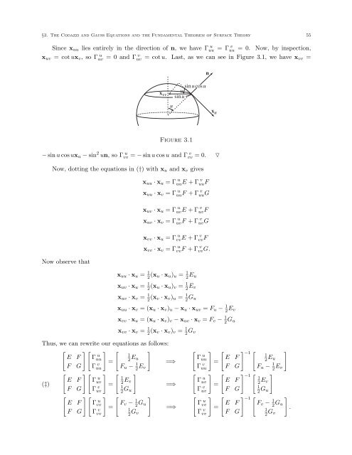
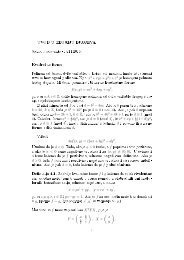
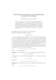
§3. The Codazzi and Gauss Equations and the Fundamental Theorem of Surface Theory 55Since x uu lies entirely in the direction of n, wehave Γuu u =Γuu v =0. Now, byinspection,x uv = cot ux v ,soΓuv u =0and Γuv v = cot u. Last, as we can see in Figure 3.1, we have x vv =nx vvsin u cos uusin uux uFigure 3.1− sin u cos ux u − sin 2 un, soΓ uvv = − sin u cos u and Γ vvv =0.▽Now, dotting the equations in (†) with x u and x v givesx uu · x u =ΓuuE u +ΓuuFvx uu · x v =ΓuuF u +ΓuuGvx uv · x u =ΓuvE u +ΓuvFvx uv · x v =ΓuvF u +ΓuvGvNow observe thatx vv · x u =Γ uvvE +Γ vvvFx vv · x v =Γ uvvF +Γ vvvG.x uu · x u = 1 2 (x u · x u ) u = 1 2 E ux uv · x u = 1 2 (x u · x u ) v = 1 2 E vx uv · x v = 1 2 (x v · x v ) u = 1 2 G ux uu · x v =(x u · x v ) u − x u · x uv = F u − 1 2 E vx vv · x u =(x u · x v ) v − x uv · x v = F v − 1 2 G ux vv · x v = 1 2 (x v · x v ) v = 1 2 G vThus, we can rewrite our equations as follows:[ ][ ] [ ]E F Γuuu 1F G Γuuv =2 E uF u − 1 2 E =⇒v[ ][ ] [ ]E F Γuvu 1F G Γuvv =2 E v(‡)12 G =⇒u[ ][ ] [ ]E F Γvvu F v − 1F G Γvvv =2 G u12 G =⇒v[Γ u uuΓ v uu[Γ u uvΓ v uv[Γ uvvΓ vvv]=[E=F] [E=F] [EF] −1 [ ]1F2 E uG F u − 1 2 E v] −1 [ ]F 12 E v1G2 G u] −1 [ ]F F v − 1 2 G u1G2 G .v
Page 1:
DIFFERENTIALGEOMETRY:A First Course
Page 6 and 7: 4 Chapter 1. Curves2πb2πaFigure 1
Page 8 and 9: 6 Chapter 1. CurvesAlternatively, s
Page 10 and 11: 8 Chapter 1. CurvesAn important obs
Page 12 and 13: 10 Chapter 1. Curvesof the road, st
Page 14 and 15: 12 Chapter 1. CurvesSummarizing,κ(
Page 16 and 17: 14 Chapter 1. Curvescurvature κ. I
Page 18 and 19: 16 Chapter 1. CurvesFigure 2.2Conve
Page 20 and 21: 18 Chapter 1. Curvesalso Exercise 2
Page 22 and 23: 20 Chapter 1. Curvesto the curve β
Page 24 and 25: 22 Chapter 1. Curvesthe osculating
Page 26 and 27: 24 Chapter 1. CurvesWe turn now to
Page 28 and 29: 26 Chapter 1. Curvesintersect C eit
Page 30 and 31: 28 Chapter 1. Curvesh(s,t)α(t)α(s
Page 32 and 33: 30 Chapter 1. Curvesy( x(s) ,y(s))
Page 34 and 35: 32 Chapter 1. Curvesɛ2ɛ 1ɛ 3CFig
Page 36 and 37: CHAPTER 2Surfaces: Local Theory1. P
Page 38 and 39: 36 Chapter 2. Surfaces: Local Theor
Page 78 and 79: 76 Chapter 3. Surfaces: Further Top
Page 102 and 103: 100 Chapter 3. Surfaces: Further To
Page 104 and 105: 102 Chapter 3. Surfaces: Further To
Page 106 and 107:
104 Chapter 3. Surfaces: Further To
Page 108 and 109:
106 Chapter 3. Surfaces: Further To
Page 110 and 111:
108 Appendix. Review of Linear Alge
Page 112 and 113:
Page 114 and 115:
Page 116 and 117:
ANSWERS TO SELECTED EXERCISES1.1.1
Page 118 and 119:
116 SELECTED ANSWERS2.4.8 Only circ
Page 120:
118 INDEXisometry, 107K, 48k-point
show all

DIFFERENTIAL GEOMETRY: A First Course in Curves and Surfaces

You also want an ePaper? Increase the reach of your titles

Delete template?

Save as template?