DIFFERENTIAL GEOMETRY: A First Course in Curves and Surfaces

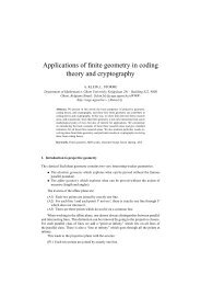
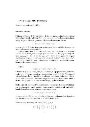
16 Chapter 1. CurvesFigure 2.2Conversely, if τ/κ is constant, set τ/κ = cot θ for some angle θ ∈ (0,π). Set A(s) =cos θT(s)+sin θB(s). Then A ′ (s) =(κ cos θ − τ sin θ)N(s) =0, soA(s) isaconstant unit vector A, andT(s) · A = cos θ is constant, as desired. □Example 5. In Example 3 we saw a curve α with κ = τ, sofrom the proof of Proposition 2.5 wesee that the curve should make a constant angle θ = π/4 with the vector A = 1 √2(T+B) =(0, 0, 1)(as should have been obvious from the formula for T alone). We verify this in Figure 2.3 by drawingα along with the vertical cylinder built on the projection of α onto the xy-plane. ▽Figure 2.3