DIFFERENTIAL GEOMETRY: A First Course in Curves and Surfaces

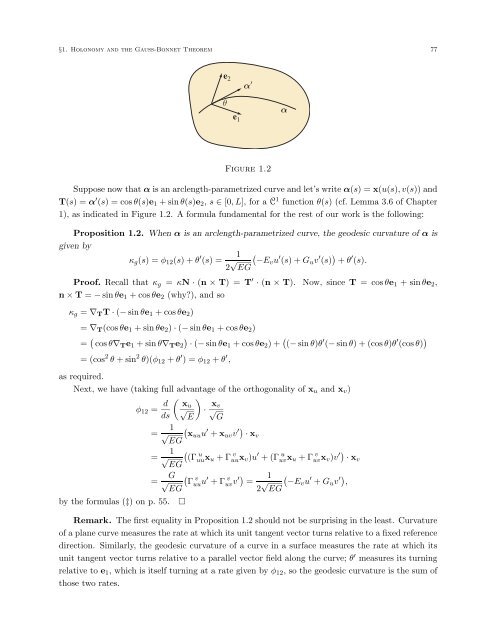
§1. Holonomy and the Gauss-Bonnet Theorem 77e 2α ′θe 1αFigure 1.2Suppose now that α is an arclength-parametrized curve and let’s write α(s) =x(u(s),v(s)) andT(s) =α ′ (s) =cos θ(s)e 1 + sin θ(s)e 2 , s ∈ [0,L], for a C 1 function θ(s) (cf. Lemma 3.6 of Chapter1), as indicated in Figure 1.2. A formula fundamental for the rest of our work is the following:Proposition 1.2. When α is an arclength-parametrized curve, the geodesic curvature of α isgiven byκ g (s) =φ 12 (s)+θ ′ 1(s) =2 √ (−Ev u ′ (s)+G u v ′ (s) ) + θ ′ (s).EGProof. Recall that κ g = κN · (n × T) =T ′ · (n × T). Now, since T = cos θe 1 + sin θe 2 ,n × T = − sin θe 1 + cos θe 2 (why?), and soκ g = ∇ T T · (− sin θe 1 + cos θe 2 )= ∇ T (cos θe 1 + sin θe 2 ) · (− sin θe 1 + cos θe 2 )= ( cos θ∇ T e 1 + sin θ∇ T e 2)· (− sin θe1 + cos θe 2 )+ ( (− sin θ)θ ′ (− sin θ)+(cos θ)θ ′ (cos θ) )= (cos 2 θ + sin 2 θ)(φ 12 + θ ′ )=φ 12 + θ ′ ,as required.Next, we have (taking full advantage of the orthogonality of x u and x v )φ 12 = d ( )xu x√ · √ vds E Gby the formulas (‡) onp.55.= 1 √EG(xuu u ′ + x uv v ′) · x v= 1 √EG((Γuuu x u +Γ v uux v )u ′ +(Γ u uvx u +Γ v uvx v )v ′) · x v= G √EG(Γvuu u ′ +Γ v uvv ′) =□12 √ EG(−Ev u ′ + G u v ′) ,Remark. The first equality in Proposition 1.2 should not be surprising in the least. Curvatureof a plane curve measures the rate at which its unit tangent vector turns relative to a fixed referencedirection. Similarly, the geodesic curvature of a curve in a surface measures the rate at which itsunit tangent vector turns relative to a parallel vector field along the curve; θ ′ measures its turningrelative to e 1 , which is itself turning at a rate given by φ 12 ,sothe geodesic curvature is the sum ofthose two rates.