Transformada de Fourier

More documents

Recommendations

Info

2.5. Propiedades de la transformada de Fourier 129donde x r (t) es la parte real de x (t) y x i (t) es la parte imaginaria de x (t), la transformadade Fourier resultaEntonces,X ( f ) ==R ( f ) =Z ∞−∞Z ∞−∞Z ∞−j[x r (t) + jx i (t)] e −j2π f t dt[x r (t) cos (2π f t) + x i (t) sen (2π f t)] dt−∞= R ( f ) + jI ( f ) .Z ∞I ( f ) = −−∞Z ∞[x r (t) sen (2π f t) − x i (t) cos (2π f t)] dt[x r (t) cos (2π f t) + x i (t) sen (2π f t)] dt,−∞[x r (t) sen (2π f t) − x i (t) cos (2π f t)] dt.De manera análoga, la fórmula de síntesis para funciones complejas permite obtenerx r (t) =Z ∞x i (t) = −−∞Z ∞[R ( f ) cos (2π f t) − I ( f ) sen (2π f t)] d f ,−∞[R ( f ) sen (2π f t) + I ( f ) cos (2π f t)] d f .Si x (t) es real, entonces x (t) = x r (t) [x i (t) ≡ 0], y las partes real e imaginaria de lastransformada de Fourier sonR e ( f ) =Z ∞I o ( f ) = −−∞Z ∞x r (t) cos (2π f t) dt, (2.77)−∞x r (t) sen (2π f t) dt. (2.78)En este caso, R e ( f ) es una función par (de la frecuencia) ya que R e ( f ) = R e (− f );análogamente, como I o ( f ) = −I o (− f ), la transformada I o ( f ) es impar.Si x (t) es imaginaria pura, x (t) = jx i (t) [x r (t) ≡ 0], y entoncesR o ( f ) =I e ( f ) =Z ∞−∞Z ∞−∞x i (t) sen (2π f t) dt, (2.79)x i (t) cos (2π f t) dt. (2.80)Ahora, R o ( f ) es una función impar de la frecuencia, e I e ( f ) es una función par. En laTabla 2.4 se listan diferentes propiedades de simetría de funciones temporales complejasy las características de sus correspondientes transformadas de Fourier.EJEMPLO 2.30. Determinación simultánea de la transformada de dos funciones realesSe pueden utilizar las relaciones (2.77)-(2.80) para determinar simultáneamente la transformada deFourier de dos señales reales. Para ilustrar esto, consideremos dos funciones reales x (t) y y (t).Procesamiento Digital de Señales U.N.S. 2011
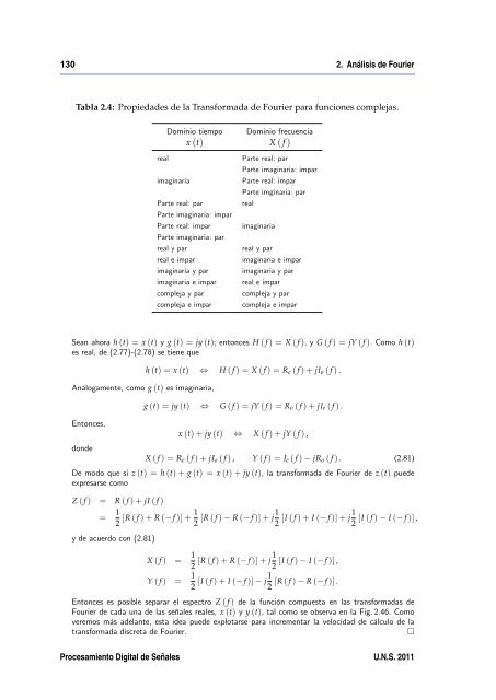
130 2. Análisis de FourierTabla 2.4: Propiedades de la Transformada de Fourier para funciones complejas.Dominio tiempo Dominio frecuenciax (t) X ( f )realimaginariaParte real: parParte imaginaria: imparParte real: imparParte imaginaria: parreal y parreal e imparimaginaria y parimaginaria e imparcompleja y parcompleja e imparParte real: parParte imaginaria: imparParte real: imparParte imginaria: parrealimaginariareal y parimaginaria e imparimaginaria y parreal e imparcompleja y parcompleja e imparSean ahora h (t) = x (t) y g (t) = jy (t); entonces H ( f ) = X ( f ), y G ( f ) = jY ( f ). Como h (t)es real, de (2.77)-(2.78) se tiene queAnálogamente, como g (t) es imaginaria,Entonces,dondeh (t) = x (t) ⇔ H ( f ) = X ( f ) = R e ( f ) + jI o ( f ) .g (t) = jy (t) ⇔ G ( f ) = jY ( f ) = R o ( f ) + jI e ( f ) .x (t) + jy (t) ⇔ X ( f ) + jY ( f ) ,X ( f ) = R e ( f ) + jI o ( f ) , Y ( f ) = I e ( f ) − jR o ( f ) . (2.81)De modo que si z (t) = h (t) + g (t) = x (t) + jy (t), la transformada de Fourier de z (t) puedeexpresarse comoZ ( f ) = R ( f ) + jI ( f )= 1 2 [R ( f ) + R (− f )] + 1 2 [R ( f ) − R (− f )] + j 1 2 [I ( f ) + I (− f )] + j 1 [I ( f ) − I (− f )] ,2y de acuerdo con (2.81)X ( f ) = 1 2 [R ( f ) + R (− f )] + j 1 [I ( f ) − I (− f )] ,2Y ( f ) = 1 2 [I ( f ) + I (− f )] − j 1 [R ( f ) − R (− f )] .2Entonces es posible separar el espectro Z ( f ) de la función compuesta en las transformadas deFourier de cada una de las señales reales, x (t) y y (t), tal como se observa en la Fig. 2.46. Comoveremos más adelante, esta idea puede explotarse para incrementar la velocidad de cálculo de latransformada discreta de Fourier.Procesamiento Digital de Señales U.N.S. 2011
Page 1 and 2: 82 2. Análisis de FourierFig. 2.9.
Page 3 and 4: 84 2. Análisis de FourierFig. 2.11
Page 13 and 14: 94 2. Análisis de Fourierfunción
Page 25: 106 2. Análisis de FourierHaciendo
Page 28 and 29: 2.4. Señales periódicas y la tran
Page 36 and 37: 2.5. Propiedades de la transformada

Transformada de Fourier

You also want an ePaper? Increase the reach of your titles

Delete template?

Save as template?