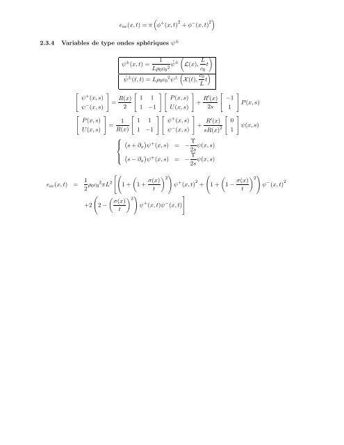
2.3 Variables d’états2.3.1 Variables <strong>de</strong> KirchoffP (x, t) = 1 (ρ 0 c ˜P L(x), L )t2 0 c 0(˜P (l, t) =ρc 2 0 P X (l), c )0L t⎧⎨⎩2.3.2 Variables <strong>de</strong> type on<strong>de</strong>s planes p ±e ac (x, t) = 1 2 R(x)2 [(1+ R c 2(1U(x, t) =c 0 L 2 S ( L(x) ) Ũ L(x), L )tc 0) (Ũ(l, t) =c 0 ˜S( X (l) U X (l), c )0L t∂x 2 P (x, (x)t)+2R′ R(x) ∂ x P (x, t) − ∂t 2 P (x, t) = 0∂ t U(x, t)+∂ x P (x, t) = 0{ []()s 2 +Υ− ∂x2 R(x)P (x, s) = 0sU(x, s)+∂ x P (x, s) = 0e ac (x, t) =πR(x) 2 P (x, t) 2 + U(x, t) 2p ± (x, t) = 1 (ρ 0 c 2 ˜p± L(x), L )t0 ( c 0˜p ± (l, t) =ρ 0 c 2 0 p ± X (l), c )0L t[ ] [ ][ ]p + (x, s)p − = 1 1 S(x)/Sc P (x, s)(x, s) 2 1 −S(x)/S c U(x, s)[ ] [][ ]P (x, s) 1 1 p + (x, s)=U(x, s) S c /S(x) −S c /S(x) p − (x, s)R(x) 2 ) (p + (x, t) 2 + p − (x, t) 2) +22.3.3 Variables <strong>de</strong> type on<strong>de</strong>s sphériques φ ±2(1 − R c 2 )]R(x) 2 p + (x, t)p − (x, t)(φ ± 1(x, t) =Lρ 0 c ˜φ ± L(x), L )t2 0 c 0˜φ ( ± (l, t) =Lρ 0 c 2 0 φ ± X (l), c )0L t[ ] [ ][φ + (x, sφ − = R(x) 1 1 P (x, s)(x, s) 2 1 −1 U(x, s)[ ] [ ][P (x, s)= 1 1 1 φ + (x, s)U(x, s) R(x) 1 −1 φ − (x, s)]]{ (s + ∂x)φ + (x, s) = σ(x)φ − (x, s)(s − ∂x)φ − (x, s) = −σ(x)φ + (x, s)
e ac (x, t) =π(φ + (x, t) 2 + φ − (x, t) 2)2.3.4 Variables <strong>de</strong> type on<strong>de</strong>s sphériques ψ ±(ψ ± 1(x, t) =Lρ 0 c ˜ψ ± L(x), L )t2 0 c 0˜ψ ( ± (l, t) =Lρ 0 c 2 0 ψ ± X (l), c )0L t[ ] [ ][ ]ψ + (x, s)ψ − = R(x) 1 1 P (x, s)(x, s) 2 1 −1 U(x, s)[ ] [ ][ ]P (x, s)= 1 1 1 ψ + (x, s)U(x, s) R(x) 1 −1 ψ − (x, s)⎧⎪⎨+ R′ (x)2s+ R′ (x)sR(x) 2 [01( )s + ∂x ψ + (x, s) = − Υ ψ(x, s)2s[ ]−1P (x, s)1]ψ(x, s)⎪⎩( )s − ∂x ψ + (x, s) = − Υ ψ(x, s)2se ac (x, t) = 1 (2 ρ 0c 2 0 πL[(1+2 1+ σ(x) ) ) 2ψ + (x, t) 2 +t( ( ) )]σ(x)2+2 2 −ψ + (x, t)ψ − (x, t)t(1+(1 − σ(x) ) ) 2ψ − (x, t) 2t
- Page 1 and 2:
Rapport de stage - Master 2 SAR ATI
- Page 4 and 5: Table des matièresIntroduction 4Co
- Page 6: IntroductionContexte et état de l
- Page 10 and 11: 1 Cas des tubes droits sans pertes1
- Page 12 and 13: 1.2 Transposition de la méthode po
- Page 14 and 15: oùDans le domaine de Laplace, le m
- Page 16 and 17: Υ = −40.30.2R(l) et −R(l)0.10
- Page 18 and 19: 4 Adimensionnement, convention axia
- Page 20 and 21: La convention appelée “conventio
- Page 22 and 23: 1.5Υ < 010.50−0.5 −0.4 −0.3
- Page 24 and 25: oùQ(s) =[][[1, σ l ]∆(s) [0,−
- Page 26 and 27: Ces valeurs propres et la matrice d
- Page 28 and 29: 6.3 Etudes et interprétation des v
- Page 30 and 31: ΥTubes symétriquesGéométrie de
- Page 32 and 33: Υ = 2, θ = 2, R l = 0.1, ε = 0
- Page 34 and 35: (θ = 0,ε = 0) Υ = 10 Υ = 1 Υ =
- Page 36 and 37: (θ = ln(2),ε = 0) Υ = 10 Υ = 1
- Page 38 and 39: (θ = ln(10),ε = 0) Υ = 10 Υ = 1
- Page 40 and 41: (θ = 0,ε = 0.1) Υ = 10 Υ = 1 Υ
- Page 42 and 43: (θ = ln(2),ε = 0.1) Υ = 10 Υ =
- Page 44 and 45: (θ = ln(10),ε = 0.1) Υ = 10 Υ =
- Page 46 and 47: Ces nombreuses figures nous donnent
- Page 48 and 49: Conclusion et perspectivesNous avon
- Page 50 and 51: [20] H. Haddar, Th. Hélie, and D.
- Page 52 and 53: 2 Adimensionnementl ∈ [a, b] ↦
- Page 56 and 57: 3 Convention “tronçon”3.1 Pré
- Page 58 and 59: 3.3 Quadripôles de conversionP l1p
- Page 60 and 61: φ inl(s)T + φ (s)φ outr (s)R l
- Page 62 and 63: 4 Connexion de deux tubes4.1 Connex
- Page 64 and 65: 4.3 Connexion à régularité quelc
- Page 66 and 67: 6 Forme standard réduite et applic
- Page 68 and 69: 6.3.1 Connexion (au moins C 0 ) de
- Page 70 and 71: 10ème Congrès Français d’Acous
- Page 72 and 73: où Υ = R ′′ /R. Si R est deux
- Page 74 and 75: 4 Applications et comparaisonsNous