Rapport de stage - Master 2 SAR ATIAM - Base des articles ...

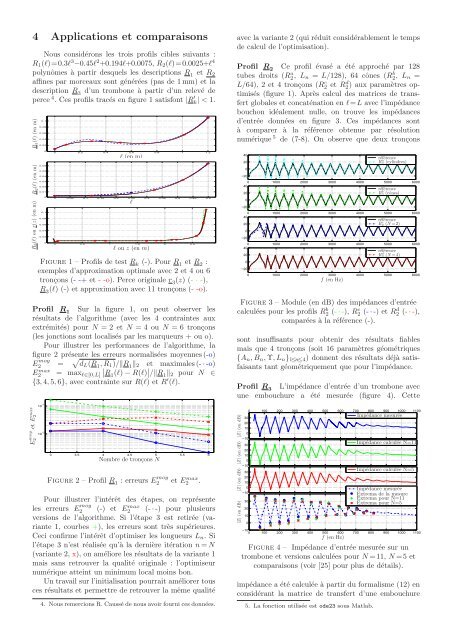
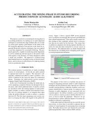
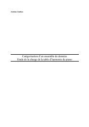
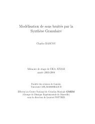
4 Applications et comparaisonsNous considérons les trois profils cibles suivants :R 1 (l)=0.3l 3 −0.45l 2 +0.194l+0.0075, R 2 (l)=0.0025+l 4polynômes à partir desquels les descriptions R 1 et R 2affines par morceaux sont générées (pas de 1mm) et ladescription R 3 d’un trombone à partir d’un relevé deperce 4 . Ces profils tracés en figure 1 satisfont |R ′ k| < 1.R 1 (l) (en m)R 2 (l) (en m)R3(l) ou r(z) (en m)0.10.080.060.040.0200.060.050.040.030.020.0100.10.080.060.040.020l (en m)0 0.2 0.4 0.6 0.8 1 1.2l0 0.05 0.1 0.15 0.2 0.25 0.3 0.35 0.4 0.45 0.5l ou z (en m)0 0.5 1 1.5 2 2.5Figure 1 – Profils de test R k (-). Pour R 1 et R 2 :exemples d’approximation optimale avec 2 et 4 ou 6tronçons (- -+ et - -o). Perce originale r 3 (z) (- · -),R 3 (l) (-) et approximation avec 11 tronçons (- -o).Profil R 1 Sur la figure 1, on peut observer lesrésultats de l’algorithme (avec les 4 contraintes auxextrémités) pour N = 2 et N = 4 ou N = 6 tronçons(les jonctions sont localisés par les marqueurs + ou o).Pour illustrer les performances de l’algorithme, lafigure 2 présente les erreurs normalisées moyennes(-o)E moy2 = √ d L (R 1 ,R ∣ 1 )/‖R 1 ‖ 2 et maximales(-·-o)E2 max = max l∈[0,L] R 1 (l)−R(l) ∣ ∣/‖R 1 ‖ 2 pour N ∈{3,4,5,6}, avec contrainte sur R(l) et R ′ (l).avec la variante 2 (qui réduit considérablement le tempsde calcul de l’optimisation).Profil R 2 Ce profil évasé a été approché par 128tubes droits (R a 2, L n = L/128), 64 cônes (R b 2, L n =L/64), 2 et 4 tronçons (R c 2 et R d 2) aux paramètres optimisés(figure 1). Après calcul des matrices de transfertglobales et concaténation en l=L avec l’impédancebouchon idéalement nulle, on trouve les impédancesd’entrée données en figure 3. Ces impédances sontà comparer à la référence obtenue par résolutionnumérique 5 de (7-8). On observe que deux tronçons40200−200 1000 2000 3000 4000 5000 600040référence20R2 b (cônes)0−200 1000 2000 3000 4000 5000 600040référence20R2 c (N=2)0−200 1000 2000 3000 4000 5000 600040référence20R2 d (N=4)0−200 1000 2000 3000 4000 5000 6000f (en Hz)référenceR a 2 (cylindres)Figure 3 – Module (en dB) des impédances d’entréecalculées pour les profils R b 2 (-·-), R c 2 (-·-) et R d 2 (-·-),comparées à la référence (-).sont insuffisants pour obtenir des résultats fiablesmais que 4 tronçons (soit 16 paramètres géométriques{A n ,B n ,Υ,L n } 1≤n≤4 ) donnent des résultats déjà satisfaisantstant géométriquement que pour l’impédance.Profil R 3 L’impédance d’entrée d’un trombone avecune embouchure a été mesurée (figure 4). CetteE moyet E max2 2max10 −110 −2Nombre de tronçons N3 3.5 4 4.5 5 5.5 6Figure 2 – Profil R 1 : erreurs E moy2 et E max2 .Pour illustrer l’intérêt des étapes, on représenteles erreurs E moy2 (-) et E2 max (-·-) pour plusieursversions de l’algorithme. Si l’étape 3 est retirée (variante1, courbes +), les erreurs sont très supérieures.Ceci confirme l’intérêt d’optimiser les longueurs L n . Sil’étape 3 n’est réalisée qu’à la dernière itération n=N(variante 2, x), on améliore les résultats de la variante 1mais sans retrouver la qualité originale : l’optimiseurnumérique atteint un minimum local moins bon.Un travail sur l’initialisation pourrait améliorer tousces résultats et permettre de retrouver la même qualité4. Nous remercions R. Caussé de nous avoir fourni ces données.|Z| (en dB)|Z| (en dB)|Z| (en dB)|Z| (en dB)3020100−103020100−103020100−1030201000 100 200 300 400 500 600 700 800 900 1000 1100−100 100 200 300 400 500 600 700 800 900 1000 1100f (en Hz)Impédance mesuréeImpédance calculée N=11Impédance calculée N=5Impédance mesuréeExtrema de la mesureExtrema pour N=11Extrema pour N=5Figure 4 – Impédance d’entrée mesurée sur untrombone et versions calculées pour N=11, N=5 etcomparaisons (voir [25] pour plus de détails).impédance a été calculée à partir du formalisme (12) enconsidérant la matrice de transfert d’une embouchure5. La fonction utilisée est ode23 sous Matlab.