Молодой учёный

“Young Scientist” . #3 (50) . March 2013 Mathematics
For other two parts of the boundary we use the same way to calculate the integrals and get
A2
∫( rr , u) ⋅ndΓ= ∫( rr , u) ⋅( -1, 0) dΓ= ∫ r( tk 1,
x) dx,
A
-
1
Γ3 Γ3
dΓ
( rr , u) ⋅ndΓ= ( rr , u) ⋅( u,
- 1) = 0.
2
u + 1
∫ ∫
Γ4 Γ4
Combine (5) – (7) and (9) – (11):
⎛∂r ∂(
ru)
⎞
x2 A2
0 = ∫⎜ + ⎟dG
= ( rr , u) ⋅ndΓ=- r( tk, x) dx + r( tk 1,
x) dx.
t x
x1 A
-
∂ ∂ ∫ ∫ ∫ 1
G ⎝ ⎠ Γ
It implies (4).
3. Simple semi-discrete approximation
Now take integer n > 2 and construct uniform mesh in x with nodes x = ih, i = 0, ±1, ± 2,…,
i ..., and meshsize h =1 n. Let we
h
know the (approximate) solution r ( tk- 1,
x)
at time level tk - 1 and construct the approximate solution at time level t k.
Integrals
of solution in a small vicinities of each point xi may be some useful intermediate data. For example, let construct integrals
xi+
12 h
i ≡ ∫ r
x
k
i-12
I ( t , x) dx
[ x , x ].
at each interval i- 12 i+
12
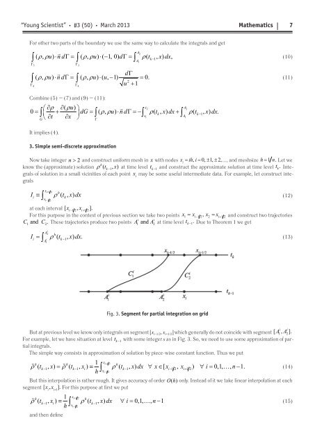
For this purpose in the context of previous section we take two points x1xi- 12, x2xi+ 12
i i
1 and 2.
A and A at time level 1 . k
C C These trajectories produce two points 1 2
i
A2
h
i = ∫ r i
A
k-1
1
I ( t , x) dx.
Fig. 3. Segment for partial integration on grid
7
(10)
(11)
(12)
= = and construct two trajectories
t - Due to Theorem 1 we get
i i
But at previous level we know only integrals on segment [xi–1/2, xi+1/2] which generally do not coincide with segment [ A1, A 2].
For example, let we have situation at level tk - 1 with some integer s as in Fig. 3. So, we need to use some approximation of partial
integrals.
The simple way consists in approximation of solution by piece-wise constant function. Thus we put
1 x
h h i+
12 h
r ( tk-1, x) = r ( tk-1, xi) ≡ r ( tk1, x) dx x [ xi 12, xi 12)
i 0,1, , n 1.
h ∫x
- ∀ ∈ - + ∀ = -
(14)
i-12
But this interpolation is rather rough. It gives accuracy of order O(h) only. Instead of it we take linear interpolation at each
segment [x i , x i+1 ]. For this purpose at fi rst we put
1 x
h i+
12 h
r ( tk-1, xi) ≡ r ( tk1, x) dx i 0,1, , n 1
h ∫x
- ∀ = -
(15)
i-12
and then defi ne
(13)