Молодой учёный

8 Математика
«Молодой учёный» . № 3 (50) . Март, 2013 г.
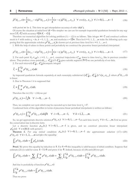
with period n for i . This time we get interpolation accuracy of order O(h 2 ).
Of course the situation at initial level (k =1) is simpler: we can use for example trapezoidal quadrature formula for any seg-
i i ii i i
ment [A , A2 ] 1 with accuracy OOh(A ( h(A - A1 ) 2 2–
- A1 ) ).
Therefore our numerical algorithm for solving problem (1) – (2) is as follows. Take integer m > 2 and construct uniform
mesh in t with nodes tk = kt, k = 0, 1, 2,...,m, and meshsize t- = T m. Then for k = 0, 1, 2,...,m make the following cycle supposing
that the approximate solution is known yet at previous time-level for i = 0, 1,...,n–1.
1. With the help of values in these points and periodicity we construct the piecewise linear (periodical) interpolant
k
2. For each point (t ,x ), i = 0, 1,…,n -1,
k i+1 2 i = 0, 1,...,n–1, construct trajectories C down to time-level t i+1 2
k–1 like in previous considerations.
They produce cross-points If goes outside segment [0,1] we use periodicity of our data.
2. For each interval compute integral
k-1
Ai+
12 h
i = ∫ r k-1
A
k-1
i-12
I ( t , x) dx
(18)
k-1 k-1
by trapezoid quadrature formula separately at each nonempty subinterval ( Ai- 12, Ai+ 12) ∩ ( xs, xs+
1)
where
is linear.
3. Due to Theorem 1 it is supposed that
I ( t , x) dx.
(19)
xi+
12 h
i ≈ ∫ r
x
k
i-12
Therefore like in (15) – (16) we put
Thus, we complete our cycle which may be executed up to last time-level t m = T.
Condensed form of this algorithm in terms of piecewise linear periodical interpolants is written as follows:
h
k-1
Ai+
12 h
k i k-1
Ai-12
k -1
r ( t , x ) = ∫ r ( t , x) dx h ∀ i = 0, , n -1, ∀ k = 1, 2, , m.
(21)
So, we get approximate discrete solution
the conservation law in discrete form.
at each time-level First we prove
Let a discrete function is given, and we construct piecewise linear interpolant
h
rinit ( x) ∀ x∈
[0,1) with period 1.
Theorem 2. For any initial condition
satisfies the equality:
the approximate solution (17)–(20)
1 1
h h
r
0
k = r
0
init
∫ ( t , x) dx ∫ ( x) dx.
(22)
Proof. We prove this equality by induction in k. For k = 0 this inequality is valid because of initial condition. Suppose that
estimate (21) is valid for some k -1≥ 0 and prove it for k. Indeed, because of (18) and (20) we get
1
∫ ∑ ∫ ∑ ∫ ∫
0
k-1 k-1
xi 12 Ai 12 A
h + h + h n-12
h
k = k = k-1 1 k 1
x
k k 1
i 12 A
- = -
i 12 A
-
- - -12
0≤≤ i n-1 0≤≤ i n-1
r ( t , x) dx r ( t , x) dx r ( t , x) dx r ( t , x) dx.
And due to periodicity of function
k-1
An-12
k-1
A-12
1
h h
k-1 =
0
k-1
∫ ∫
r ( t , x) dx r ( t , x) dx.
Thus we prove
(16)
(17)
(20)