Stefan Wirtz Vom Fachbereich VI (Geographie/Geowissenschaften ...

Experimentelle Rinnenerosionsforschung vs. Modellkonzepte – Quantifizierung der hydraulischen und erosiven Wirksamkeit von Rinnen
2.2.2 Rainfall Simulations
The test plot was circular, with a diameter of 60 cm and an area of 0.28 m 2 . It was delimited
by a steel ring of 7 cm height, which was introduced into the soil for at least 3 cm. The outlet
was V-shaped and was placed at the deepest point of the plot at surface level. The commercial
full cone nozzle (Lechler 460.608) was fed with a pressure of about 40 kPa (0.4 bars) at a
height of 2 m. The water flow was regulated by a flow metre (Type KSK-1200HIG100)
positioned on a separate pole in 1.5 m height. The resulting rainfall intensity was maintained
throughout the experiments at around 40 mm h -1 , which is considered to be mean
thunderstorm rainfall intensity with a return period of about 2 years [26]. The complete runoff
was collected and runoff and soil detachment was determined gravimetrically. [23, 27, 28, 29,
30]. The standard deviation of the rainfall intensity is < 5 % [28].
Plot surface parameters were rock fragment cover, separated in embedded and overlying,
vegetation cover, bare soil area, separated in crusted and uncrusted and finally the slope of the
plot. These parameters were optically estimated in the field and validated again with the help
of digital photographs taken from every plot, and preferably taken at an angle of 90° to the
plot surface. The slope was measured by a clinometer.
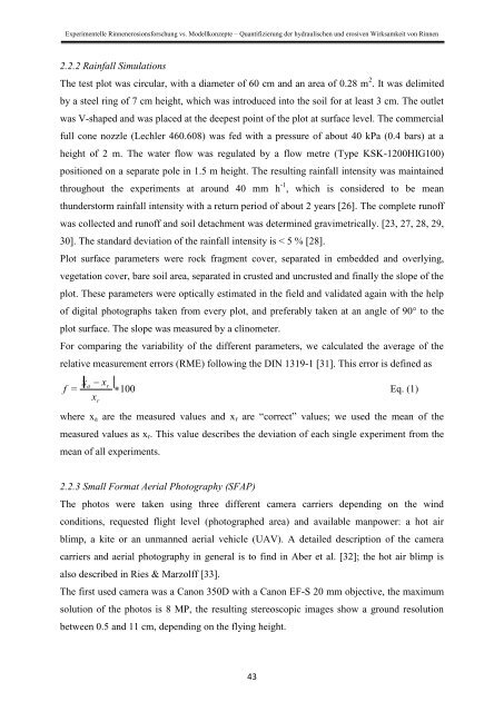
For comparing the variability of the different parameters, we calculated the average of the
relative measurement errors (RME) following the DIN 1319-1 [31]. This error is defined as
xa
xr
f = 100
Eq. (1)
x
r
where x a are the measured values and x r are “correct” values; we used the mean of the
measured values as x r . This value describes the deviation of each single experiment from the
mean of all experiments.
2.2.3 Small Format Aerial Photography (SFAP)
The photos were taken using three different camera carriers depending on the wind
conditions, requested flight level (photographed area) and available manpower: a hot air
blimp, a kite or an unmanned aerial vehicle (UAV). A detailed description of the camera
carriers and aerial photography in general is to find in Aber et al. [32]; the hot air blimp is
also described in Ries & Marzolff [33].
The first used camera was a Canon 350D with a Canon EF-S 20 mm objective, the maximum
solution of the photos is 8 MP, the resulting stereoscopic images show a ground resolution
between 0.5 and 11 cm, depending on the flying height.
43