REPORT - Search CIMMYT repository

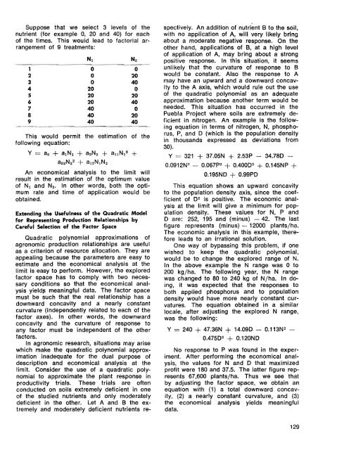
Suppose that we select 3 levels of the
nutrient (for example 0, 20 and 40) for each
of the times. This would lead to factorial arrangement
of 9 treatments:
1
2
3
4
5
6
7
8
9
o
o
20
20
20
40
40
40
o
20
40
o
20
40
o
20
40
This would permit the estimation of the
following equation:
Y = ao + a1N1 + a2N2 + allN12 +
a22N22 + a12N1N2
An economical analysis to the limit will
result in the estimation of the optimum value
of N1 and N2. In other words, both the optimum
rate and time of application would be
obtained.
Extending the Usefulness of the Quadratic Model
for Representing Production Relationships by
Careful Selection of the Factor Space
Quadratic polynomial approximations of
agronomic production relationships are useful
as a criterion of resource allocation. They are
appealing because the parameters are easy to
estimate and the economical analysis at the
limit is easy to perform. However, the explored
factor space has to comply with two necessary
conditions so that the economical analysis
yield~ meaningful data. The factor space
must be such that the real relationship has a
downward concavity and a nearly constant
curvature (independently related to each of the
factor axes). In other words, the downward
concavity and the curvature of response to
any factor must be independent of the other
factors.
In agronomic research, situations may arise
which make the quadratic polynomial approximation
inadequate for the dual purpose of
description and economical analysis at the
limit. Consider the use of a quadratic polynomial
to approximate the plant response in
productivity trials. These trials are often
conducted on soils extremely deficient in one
of the studied nutrients and only moderately
deficient in the other. Let A and B the extremely
and moderately deficient nutrients re-
spectively. An addition of nutrient B to the soil,
with no application of A, will very likely bring
about a moderate negative response. On the
other hand, applications of B, at a high level
of application of A, may bring about a strong
positive response. In this situation, it seems
unlikely that the curvature of response to B
would be constant. Also the response to A
may have an upward and a downward concavity
to the A axis, which would rule out the use
of the quadratic polynomial as an adequate
approximation because another term would be
needed. This situation has occurred in the
Puebla Project where soils are extremely deficient
in nitrogen. An example is the following
equation in terms of nitrogen, N, phosphorus,
P, and 0 (which is the population density
in thousands expressed as deviations from
30).
Y = 321 + 37.05N + 2.53P - 34.780 ­
0.0912N2 - 0.067p2 + 0.4000 2 + 0.145NP +
0.195NO + 0.99PO
This equation shows an upward concavity
to the population density axis, since the coefficient
of 0 2 is positive. The economic analysis
at the limit will give a minimum for population
density. These values for N, P and
o are: 252, 195 and (minus) - 42. The last
figure represents (minus) - 12000 plants/ha.
The economic analysis in this example, therefore
leads to an irrational solution.
One way of bypassing this problem, if one
wished to keep the quadratic polynomial,
would be to change the explored range of N.
In the above example the N range was 0 to
200 kg/ha. The following year, the N range
was changed to 80 to 240 kg of N/ha. In doing,
it was expected that the responses to
both applied phosphorus and to population
density would have more nearly constant curvatures.
The equation obtained in a similar
locale, after adjusting the explored N range,
was the following:
Y = 240 + 47.36N + 14.090 - 0.113N2 ­
0.4750 2 + O.120NO
No response to P was found in the experiment.
After performing the economical analysis,
the values for Nand 0 that maximized
profit were 180 and 37.5. The latter figure represents
67,600 plants/ha. Thus we see that
by adjusting the factor space, we obtain an
equation with (1) a total downward concavity,
(2) a nearly constant curvature, and (3)
the economical analysis yields meaningful
data.
129