- Page 2 and 3:
SUBAT MIC PHYSICS Third Edition
- Page 4 and 5:
SUBAT MIC PHYSICS Ernest M Henley A
- Page 6 and 7:
To Elaine and Viviana
- Page 8 and 9:
Acknowledgments In writing the pres
- Page 10 and 11:
Preface to the First Edition Subato
- Page 12 and 13:
Preface to the Third Edition Subato
- Page 14 and 15:
General Bibliography The reader of
- Page 16 and 17:
Contents Dedication v Acknowledgmen
- Page 18 and 19:
Contents xvii 6 Structure of Subato
- Page 20 and 21:
Contents xix 12.5 GeneralReferences
- Page 22 and 23:
Chapter 1 Background and Language H
- Page 24 and 25:
1.2. Units 3 1.2 Units Table 1.1: B
- Page 26 and 27:
1.3. Special Relativity, Feynman Di
- Page 28 and 29:
1.3. Special Relativity, Feynman Di
- Page 30 and 31:
1.4. References 9 Problems 1.1. ∗
- Page 32 and 33:
Part I Tools One of the most frustr
- Page 34 and 35:
Chapter 2 Accelerators 2.1 Why Acce
- Page 36 and 37:
2.1. Why Accelerators? 15 particle
- Page 38 and 39:
2.2. Cross Sections and Luminosity
- Page 40 and 41:
2.3. Electrostatic Generators (Van
- Page 42 and 43:
2.4. Linear Accelerators (Linacs) 2
- Page 44 and 45:
2.5. Beam Optics 23 Figure 2.8: Rec
- Page 46 and 47:
2.6. Synchrotrons 25 Figure 2.10: E
- Page 48 and 49:
2.6. Synchrotrons 27 Photo 3: The p
- Page 50 and 51:
2.7. Laboratory and Center-of-Momen
- Page 52 and 53:
2.8. Colliding Beams 31 or with Eqs
- Page 54 and 55:
2.10. Beam Storage and Cooling 33 l
- Page 56 and 57:
2.11. References 35 and in E. Byckl
- Page 58 and 59:
2.11. References 37 (b) Extreme rel
- Page 60 and 61:
Chapter 3 Passage of Radiation Thro
- Page 62 and 63:
3.2. Heavy Charged Particles 41 Fig
- Page 64 and 65:
3.2. Heavy Charged Particles 43 −
- Page 66 and 67:
3.3. Photons 45 Equation (3.2) also
- Page 68 and 69:
3.4. Electrons 47 Figure 3.8: Passa
- Page 70 and 71:
3.5. Nuclear Interactions 49 Figure
- Page 72 and 73:
3.6. References 51 3.8. A beam of 1
- Page 74 and 75:
Chapter 4 Detectors What would a ph
- Page 76 and 77:
4.1. Scintillation Counters 55 The
- Page 78 and 79:
4.2. Statistical Aspects 57 Or, to
- Page 80 and 81:
4.3. Semiconductor Detectors 59 kno
- Page 82 and 83:
4.3. Semiconductor Detectors 61 Fig
- Page 84 and 85:
4.4. Bubble Chambers 63 Photo 5: Bu
- Page 86 and 87:
4.6. Wire Chambers 65 voltage suppl
- Page 88 and 89:
4.8. Time Projection Chambers 67 Fi
- Page 90 and 91:
4.10. Calorimeters 69 Figure 4.18:
- Page 92 and 93:
4.11. Counter Electronics 71 Figure
- Page 94 and 95:
4.13. References 73 Table 4.1: Func
- Page 96 and 97:
4.13. References 75 4.6. Sketch the
- Page 98 and 99:
Part II Particles and Nuclei The si
- Page 100 and 101:
Chapter 5 The Subatomic Zoo A conve
- Page 102 and 103:
5.1. Mass and Spin. Fermions and Bo
- Page 104 and 105:
5.1. Mass and Spin. Fermions and Bo
- Page 106 and 107:
5.2. Electric Charge and Magnetic D
- Page 108 and 109:
5.3. Mass Measurements 87 Figure 5.
- Page 110 and 111:
5.3. Mass Measurements 89 Figure 5.
- Page 112 and 113:
5.3. Mass Measurements 91 Earlier,
- Page 114 and 115:
5.4. A First Glance at the Subatomi
- Page 116 and 117:
5.5. Gauge Bosons 95 Figure 5.13: A
- Page 118 and 119:
5.6. Leptons 97 to its momentum, re
- Page 120 and 121:
5.7. Decays 99 Figure 5.15: Exponen
- Page 122 and 123:
5.7. Decays 101 The function g(ω)
- Page 124 and 125:
5.8. Mesons 103 5.8 Mesons Table 5.
- Page 126 and 127:
5.9. Baryon Ground States 105 Japan
- Page 128 and 129:
5.9. Baryon Ground States 107 neutr
- Page 130 and 131:
5.10. Particles and Antiparticles 1
- Page 132 and 133:
5.10. Particles and Antiparticles 1
- Page 134 and 135:
5.11. Quarks, Gluons, and Intermedi
- Page 136 and 137:
5.11. Quarks, Gluons, and Intermedi
- Page 138 and 139:
5.11. Quarks, Gluons, and Intermedi
- Page 140 and 141:
5.12. Excited States and Resonances
- Page 142 and 143:
5.12. Excited States and Resonances
- Page 144 and 145:
5.13. Excited States of Baryons 123
- Page 146 and 147:
5.13. Excited States of Baryons 125
- Page 148 and 149:
5.13. Excited States of Baryons 127
- Page 150 and 151:
5.14. References 129 in Section 5.5
- Page 152 and 153:
5.14. References 131 5.14. Use the
- Page 154 and 155:
5.14. References 133 5.32. ∗ What
- Page 156 and 157:
Chapter 6 Structure of Subatomic Pa
- Page 158 and 159:
6.2. Rutherford and Mott Scattering
- Page 160 and 161:
6.2. Rutherford and Mott Scattering
- Page 162 and 163:
6.3. Form Factors 141 The scatterin
- Page 164 and 165:
6.4. The Charge Distribution of Sph
- Page 166 and 167:
6.4. The Charge Distribution of Sph
- Page 168 and 169:
6.5. Leptons Are Point Particles 14
- Page 170 and 171:
6.5. Leptons Are Point Particles 14
- Page 172 and 173:
6.5. Leptons Are Point Particles 15
- Page 174 and 175:
6.6. Nucleon Elastic Form Factors 1
- Page 176 and 177:
6.6. Nucleon Elastic Form Factors 1
- Page 178 and 179:
6.6. Nucleon Elastic Form Factors 1
- Page 180 and 181:
6.6. Nucleon Elastic Form Factors 1
- Page 182 and 183:
6.8. Inelastic Electron and Muon Sc
- Page 184 and 185:
6.8. Inelastic Electron and Muon Sc
- Page 186 and 187:
6.9. Deep Inelastic Electron Scatte
- Page 188 and 189:
6.10. Quark-Parton Model for Deep I
- Page 190 and 191:
6.10. Quark-Parton Model for Deep I
- Page 192 and 193:
6.10. Quark-Parton Model for Deep I
- Page 194 and 195:
6.11. More Details on Scattering an
- Page 196 and 197:
6.11. More Details on Scattering an
- Page 198 and 199:
6.11. More Details on Scattering an
- Page 200 and 201:
6.11. More Details on Scattering an
- Page 202 and 203:
6.11. More Details on Scattering an
- Page 204 and 205:
6.11. More Details on Scattering an
- Page 206 and 207:
6.11. More Details on Scattering an
- Page 208 and 209:
6.11. More Details on Scattering an
- Page 210 and 211:
6.12. References 189 Some character
- Page 212 and 213:
6.12. References 191 (c) Show that
- Page 214 and 215:
6.12. References 193 6.23. Show tha
- Page 216 and 217:
Part III Symmetries and Conservatio
- Page 218 and 219:
Chapter 7 Additive Conservation Law
- Page 220 and 221:
7.1. Conserved Quantities and Symme
- Page 222 and 223:
7.1. Conserved Quantities and Symme
- Page 224 and 225:
7.2. The Electric Charge 203 7.2 Th
- Page 226 and 227:
7.2. The Electric Charge 205 or [Q,
- Page 228 and 229:
7.3. The Baryon Number 207 antineut
- Page 230 and 231:
7.4. Lepton and Lepton Flavor Numbe
- Page 232 and 233:
7.5. Strangeness Flavor 211 all bel
- Page 234 and 235:
7.5. Strangeness Flavor 213 Positiv
- Page 236 and 237:
7.6. Additive Quantum Numbers of Qu
- Page 238 and 239:
7.7. References 217 There are also
- Page 240 and 241:
7.7. References 219 7.12. Follow th
- Page 242 and 243:
Chapter 8 Angular Momentum and Isos
- Page 244 and 245:
8.2. Symmetry Breaking by a Magneti
- Page 246 and 247:
8.4. The Nucleon Isospin 225 8.4 Th
- Page 248 and 249:
8.5. Isospin Invariance 227 magneti
- Page 250 and 251:
8.6. Isospin of Particles 229 the v
- Page 252 and 253:
8.6. Isospin of Particles 231 The a
- Page 254 and 255:
8.7. Isospin in Nuclei 233 If the e
- Page 256 and 257:
8.8. References 235 Isospin doublet
- Page 258 and 259:
8.8. References 237 8.4. Verify the
- Page 260 and 261:
Chapter 9 P , C, CP, andT In the pr
- Page 262 and 263:
9.1. The Parity Operation 241 P is
- Page 264 and 265:
9.2. The Intrinsic Parities of Suba
- Page 266 and 267:
9.2. The Intrinsic Parities of Suba
- Page 268 and 269:
9.3. Conservation and Breakdown of
- Page 270 and 271: 9.3. Conservation and Breakdown of
- Page 272 and 273: 9.3. Conservation and Breakdown of
- Page 274 and 275: 9.4. Charge Conjugation 253 “Is t
- Page 276 and 277: 9.4. Charge Conjugation 255 The π
- Page 278 and 279: 9.5. Time Reversal 257 if Tψ(t) an
- Page 280 and 281: 9.5. Time Reversal 259 found to be
- Page 282 and 283: 9.6. The Two-State Problem 261 Hami
- Page 284 and 285: 9.7. The Neutral Kaons 263 9.7 The
- Page 286 and 287: 9.7. The Neutral Kaons 265 3. The s
- Page 288 and 289: 9.7. The Neutral Kaons 267 and only
- Page 290 and 291: 9.8. The Fall of CP Invariance 269
- Page 292 and 293: 9.9. References 271 • There are t
- Page 294 and 295: 9.9. References 273 9.8. * Find inf
- Page 296 and 297: 9.9. References 275 9.27. Assume th
- Page 298 and 299: 9.9. References 277 9.39. Compare t
- Page 300 and 301: Part IV Interactions In the previou
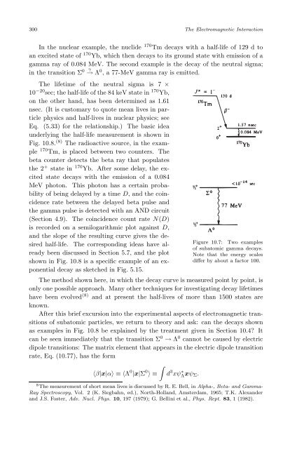
- Page 302 and 303: Chapter 10 The Electromagnetic Inte
- Page 304 and 305: 10.1. The Golden Rule 283 Schrödin
- Page 306 and 307: 10.1. The Golden Rule 285 where it
- Page 308 and 309: 10.2. Phase Space 287 Figure 10.4:
- Page 310 and 311: 10.3. The Classical Electromagnetic
- Page 312 and 313: 10.3. The Classical Electromagnetic
- Page 314 and 315: 10.4. Photon Emission 293 is a twof
- Page 316 and 317: 10.4. Photon Emission 295 the form
- Page 318 and 319: 10.4. Photon Emission 297 where V (
- Page 322 and 323: 10.5. Multipole Radiation 301 Figur
- Page 324 and 325: 10.6. Electromagnetic Scattering of
- Page 326 and 327: 10.6. Electromagnetic Scattering of
- Page 328 and 329: 10.7. Vector Mesons as Mediators of
- Page 330 and 331: 10.7. Vector Mesons as Mediators of
- Page 332 and 333: 10.8. Colliding Beams 311 10.8 Coll
- Page 334 and 335: 10.8. Colliding Beams 313 Figure 10
- Page 336 and 337: 10.9. Electron-Positron Collisions
- Page 338 and 339: 10.10. The Photon-Hadron Interactio
- Page 340 and 341: 10.10. The Photon-Hadron Interactio
- Page 342 and 343: 10.10. The Photon-Hadron Interactio
- Page 344 and 345: 10.11. Magnetic Monopoles 323 The s
- Page 346 and 347: 10.12. References 325 Quantum Elect
- Page 348 and 349: 10.12. References 327 (b) Compare t
- Page 350 and 351: 10.12. References 329 (a) How would
- Page 352 and 353: Chapter 11 The Weak Interaction Thi
- Page 354 and 355: 11.1. The Continuous Beta Spectrum
- Page 356 and 357: 11.2. Beta Decay Lifetimes 335 The
- Page 358 and 359: 11.3. The Current-Current Interacti
- Page 360 and 361: 11.3. The Current-Current Interacti
- Page 362 and 363: 11.3. The Current-Current Interacti
- Page 364 and 365: 11.4. A Variety of Weak Processes 3
- Page 366 and 367: 11.4. A Variety of Weak Processes 3
- Page 368 and 369: 11.5. The Muon Decay 347 Linac Pion
- Page 370 and 371:
11.6. The Weak Current of Leptons 3
- Page 372 and 373:
11.6. The Weak Current of Leptons 3
- Page 374 and 375:
11.7. Chirality versus Helicity 353
- Page 376 and 377:
11.9. Weak Decays of Quarks and the
- Page 378 and 379:
11.10. Weak Currents in Nuclear Phy
- Page 380 and 381:
11.10. Weak Currents in Nuclear Phy
- Page 382 and 383:
11.11. Inverse Beta Decay: Reines a
- Page 384 and 385:
11.12. Massive Neutrinos 363 11.12
- Page 386 and 387:
11.13. Majorana versus Dirac Neutri
- Page 388 and 389:
11.14. The Weak Current of Hadrons
- Page 390 and 391:
11.14. The Weak Current of Hadrons
- Page 392 and 393:
11.14. The Weak Current of Hadrons
- Page 394 and 395:
11.14. The Weak Current of Hadrons
- Page 396 and 397:
11.15. References 375 11.15 Referen
- Page 398 and 399:
11.15. References 377 11.5. Beta sp
- Page 400 and 401:
11.15. References 379 (b) * Discuss
- Page 402 and 403:
11.15. References 381 11.41. For nu
- Page 404 and 405:
Chapter 12 Introduction to Gauge Th
- Page 406 and 407:
12.1. Introduction 385 D0 ≡ 1 ∂
- Page 408 and 409:
12.2. Potentials in Quantum Mechani
- Page 410 and 411:
12.3. Gauge Invariance for Non-Abel
- Page 412 and 413:
12.3. Gauge Invariance for Non-Abel
- Page 414 and 415:
12.4. The Higgs Mechanism; Spontane
- Page 416 and 417:
12.4. The Higgs Mechanism; Spontane
- Page 418 and 419:
12.4. The Higgs Mechanism; Spontane
- Page 420 and 421:
12.4. The Higgs Mechanism; Spontane
- Page 422 and 423:
12.5. General References 401 12.5 G
- Page 424 and 425:
Chapter 13 The Electroweak Theory o
- Page 426 and 427:
13.2. The Gauge Bosons and Weak Iso
- Page 428 and 429:
13.2. The Gauge Bosons and Weak Iso
- Page 430 and 431:
13.3. The Electroweak Interaction 4
- Page 432 and 433:
13.3. The Electroweak Interaction 4
- Page 434 and 435:
13.3. The Electroweak Interaction 4
- Page 436 and 437:
13.4. Tests of the Standard Model 4
- Page 438 and 439:
13.4. Tests of the Standard Model 4
- Page 440 and 441:
13.5. References 419 Physics. 112,
- Page 442 and 443:
Chapter 14 Strong Interactions All
- Page 444 and 445:
14.1. Range and Strength of the Low
- Page 446 and 447:
14.2. The Pion-Nucleon Interaction
- Page 448 and 449:
14.2. The Pion-Nucleon Interaction
- Page 450 and 451:
14.2. The Pion-Nucleon Interaction
- Page 452 and 453:
14.3. The Form of the Pion-Nucleon
- Page 454 and 455:
14.4. The Yukawa Theory of Nuclear
- Page 456 and 457:
14.5. Low-Energy Nucleon-Nucleon Fo
- Page 458 and 459:
14.5. Low-Energy Nucleon-Nucleon Fo
- Page 460 and 461:
14.5. Low-Energy Nucleon-Nucleon Fo
- Page 462 and 463:
14.5. Low-Energy Nucleon-Nucleon Fo
- Page 464 and 465:
14.6. Meson Theory of the Nucleon-N
- Page 466 and 467:
14.7. Strong Processes at High Ener
- Page 468 and 469:
14.7. Strong Processes at High Ener
- Page 470 and 471:
14.7. Strong Processes at High Ener
- Page 472 and 473:
14.8. The Standard Model, Quantum C
- Page 474 and 475:
14.8. The Standard Model, Quantum C
- Page 476 and 477:
14.8. The Standard Model, Quantum C
- Page 478 and 479:
14.9. QCD at Low Energies 457 An ex
- Page 480 and 481:
14.10. Grand Unified Theories, Supe
- Page 482 and 483:
14.11. References 461 and Partons,
- Page 484 and 485:
14.11. References 463 Fig. 14.28 14
- Page 486 and 487:
14.11. References 465 14.25. The lo
- Page 488 and 489:
14.11. References 467 (b) What comb
- Page 490 and 491:
Part V Models “A model is like an
- Page 492 and 493:
Chapter 15 Quark Models of Mesons a
- Page 494 and 495:
15.2. Quarks as Building Blocks of
- Page 496 and 497:
15.4. Mesons as Bound Quark States
- Page 498 and 499:
15.4. Mesons as Bound Quark States
- Page 500 and 501:
15.5. Baryons as Bound Quark States
- Page 502 and 503:
15.6. The Hadron Masses 481 Figure
- Page 504 and 505:
15.7. QCD and Quark Models of the H
- Page 506 and 507:
15.7. QCD and Quark Models of the H
- Page 508 and 509:
15.7. QCD and Quark Models of the H
- Page 510 and 511:
15.7. QCD and Quark Models of the H
- Page 512 and 513:
15.8. Heavy Mesons: Charmonium, Ups
- Page 514 and 515:
15.9. Outlook and Problems 493 wher
- Page 516 and 517:
15.10. References 495 On a more adv
- Page 518 and 519:
15.10. References 497 where J± = J
- Page 520 and 521:
15.10. References 499 (b) Apply the
- Page 522 and 523:
Chapter 16 Liquid Drop Model, Fermi
- Page 524 and 525:
16.1. The Liquid Drop Model 503 Fig
- Page 526 and 527:
16.1. The Liquid Drop Model 505 Bey
- Page 528 and 529:
16.2. The Fermi Gas Model 507 N = V
- Page 530 and 531:
E/A(MeV) 16.3. Heavy Ion Reactions
- Page 532 and 533:
16.4. Relativistic Heavy Ion Collis
- Page 534 and 535:
16.4. Relativistic Heavy Ion Collis
- Page 536 and 537:
16.5. References 515 medium (i.e. s
- Page 538 and 539:
16.5. References 517 16.12. Symmetr
- Page 540 and 541:
16.5. References 519 16.25. At RHIC
- Page 542 and 543:
Chapter 17 The Shell Model The liqu
- Page 544 and 545:
17.1. The Magic Numbers 523 The res
- Page 546 and 547:
17.2. The Closed Shells 525 solved
- Page 548 and 549:
17.2. The Closed Shells 527 Figure
- Page 550 and 551:
17.3. The Spin-Orbit Interaction 52
- Page 552 and 553:
17.4. The Single-Particle Shell Mod
- Page 554 and 555:
17.5. Generalization of the Single-
- Page 556 and 557:
17.6. Isobaric Analog Resonances 53
- Page 558 and 559:
17.7. Nuclei Far From the Valley of
- Page 560 and 561:
17.8. References 539 An elementary
- Page 562 and 563:
17.8. References 541 (b) N odd. (c)
- Page 564 and 565:
Chapter 18 Collective Model Althoug
- Page 566 and 567:
18.1. Nuclear Deformations 545 spin
- Page 568 and 569:
18.2. Rotational Spectra of Spinles
- Page 570 and 571:
18.2. Rotational Spectra of Spinles
- Page 572 and 573:
18.3. Rotational Families 551 A spi
- Page 574 and 575:
18.3. Rotational Families 553 2. Th
- Page 576 and 577:
18.4. One-Particle Motion in Deform
- Page 578 and 579:
18.4. One-Particle Motion in Deform
- Page 580 and 581:
18.5. Vibrational States in Spheric
- Page 582 and 583:
18.5. Vibrational States in Spheric
- Page 584 and 585:
18.6. The Interacting Boson Model 5
- Page 586 and 587:
18.7. Highly Excited States; Giant
- Page 588 and 589:
18.8. Nuclear Models—Concluding R
- Page 590 and 591:
18.8. Nuclear Models—Concluding R
- Page 592 and 593:
18.9. References 571 J. S. Vaagen,
- Page 594 and 595:
18.9. References 573 18.13. Verify
- Page 596 and 597:
18.9. References 575 18.33. Conside
- Page 598 and 599:
18.9. References 577 18.51. (a) In
- Page 600 and 601:
Chapter 19 Nuclear and Particle Ast
- Page 602 and 603:
19.1. The Beginning of the Universe
- Page 604 and 605:
19.1. The Beginning of the Universe
- Page 606 and 607:
19.2. Primordial Nucleosynthesis 58
- Page 608 and 609:
19.3. Stellar Energy and Nucleosynt
- Page 610 and 611:
19.3. Stellar Energy and Nucleosynt
- Page 612 and 613:
19.3. Stellar Energy and Nucleosynt
- Page 614 and 615:
19.4. Stellar Collapse and Neutron
- Page 616 and 617:
19.4. Stellar Collapse and Neutron
- Page 618 and 619:
19.5. Cosmic Rays 597 We are consta
- Page 620 and 621:
19.5. Cosmic Rays 599 Figure 19.11:
- Page 622 and 623:
19.6. Neutrino Astronomy and Cosmol
- Page 624 and 625:
19.8. References 603 baryon excess
- Page 626 and 627:
19.8. References 605 Neutron Stars
- Page 628 and 629:
19.8. References 607 (a) What is th
- Page 630 and 631:
Index Abundance, 585-586 Accelerato
- Page 632 and 633:
Index 611 drift chambers, 66-67 ele
- Page 634 and 635:
Index 613 diagrams, 279 electromagn
- Page 636 and 637:
Index 615 outlook, 567 Nuclear stru
- Page 638 and 639:
Index 617 poles, 494 recurrences, 4
- Page 640 and 641:
Index 619 TCP theorem, 269, 448 Tem