CEPAL Review no. 124

CEPAL Review N° 124 • April 2018 153
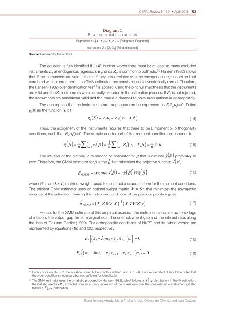
Diagram 1
Regressors and instruments
Regressors X = [X 1
X 2
] = [X 1
Z 2
] = [Endogenous Exogenous]
Instruments Z = [Z 1
Z 2
] [Exluded Included]
Source: Prepared by the authors.
The equation is fully identified if L≥K; in other words there must be at least as many excluded
instruments L 1
as endogenous regressors K 1
, since Z 2
is common to both lists. 20 Hansen (1982) shows
that, if the instruments are valid —that is, if they are correlated with the endogenous regressors and not
correlated with the error term— the GMM estimators are consistent and asymptotically normal. Therefore,
the Hansen (1982) overidentification test 21 is applied, using the joint null hypothesis that the instruments
are valid and the Z 1
instruments were correctly excluded in the estimation process. If H 0
is not rejected,
the instruments are considered valid and the model is deemed to have been estimated appropriately.
The assumption that the instruments are exogenous can be expressed as E(Z i
,u i
) = 0. Define
g i
(β ) as the function (L x 1):
Thus, the exogeneity of the instruments requires that there to be L moment or orthogonality
conditions, such that E(g i
(β)) = 0. The sample counterpart of that moment condition corresponds to:
(14)
(15)
The intuition of the method is to choose an estimator for b that minimizes preferably to
zero. Therefore, the GMM estimator for b is the that minimizes the objective function :
(16)
where W is an (L x L) matrix of weights used to construct a quadratic form for the moment conditions.
The efficient GMM estimator uses an optimal weight matrix W = S -1 that minimizes the asymptotic
variance of the estimator. Deriving the first-order conditions of the previous problem gives:
Hence, for the GMM estimate of this empirical exercise, the instruments include up to six lags
of inflation, the output gap, firms’ marginal cost, the unemployment gap and the interest rate, along
the lines of Galí and Gertler (1999). The orthogonality conditions of NKPC and its hybrid version are
represented by equations (19) and (20), respectively:
(17)
(18)
(19)
20
Order condition. If L = K, the equation is said to be exactly identified; and, if L > K, it is overidentified. It should be noted that
the order condition is necessary, but not sufficient for identification.
21
The GMM estimator uses the J-statistic proposed by Hansen (1982), which follows a distribution. In the IV estimation,
the statistic used is nR 2 , extracted from an auxiliary regression of the IV residuals over the complete set of instruments; it also
follows a distribution.
Elano Ferreira Arruda, Maria Thalita Arruda Oliveira de Olivindo and Ivan Castelar