CEPAL Review no. 124
April 2018
April 2018

You also want an ePaper? Increase the reach of your titles
YUMPU automatically turns print PDFs into web optimized ePapers that Google loves.
<strong>CEPAL</strong> <strong>Review</strong> N° <strong>124</strong> • April 2018 155<br />
Expectations<br />
Perfect forecast<br />
Focus forecast<br />
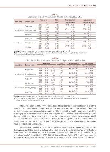
Table 3<br />
Estimation of the New Keynesian Phillips curve with HAC-GMM<br />
Business cycles<br />
Parameters J-test Heterocedasticity Autocorrelation<br />
λ γ f Hansen Pagan and Hall Cumby and Huizinga<br />
Marginal cost<br />
0.30 0.39 4.03 X 2 (5) = 29.12 X 2 (1) = 6.92<br />
(0.01) (0.00) (0.25) (0.00) (0.00)<br />
Unemployment gap<br />
-0.41 0.34 7.97 X 2 (14) = 21.14 X 2 (1) = 12.10<br />
(0.04) (0.01) (0.78) (0.04) (0.00)<br />
Output gap a -1.97 0.59 4.43 X 2 (5) = 15.54 X 2 (1) = 0.25 a<br />
(0.00) (0.01) (0.22) (0.00) (0.62)<br />
Marginal cost<br />
0.38 1.09 3.23 X 2 (5) = 20.19 X 2 (1) = 43.13<br />
(0.00) (0.00) (0.35) (0.00) (0.00)<br />
Unemployment gap<br />
-0.91 1.23 7.82 X 2 (15) = 27.13 X 2 (1) = 43.13<br />
(0.00) (0.00) (0.85) (0.02) (0.00)<br />
Output gap<br />
-0.24 1.27 5.87 X 2 (15) = 23.55 X 2 (15) = 46.94<br />
(0.52) (0.00) (0.95) (0.05) (0.00)<br />
Source: Prepared by the authors on the basis of the equation .<br />
Note: P-value in parentheses. The autocorrelation and heteroscedasticity tests were applied in the IV estimation.<br />
a<br />
Model corrected for heteroscedasticity only.<br />
Expectations<br />
Perfect forecast<br />
FOCUS forecast<br />
Table 4<br />
Estimation of the hybrid New-Keynesian Phillips curve with HAC-GMM<br />
Business cycles<br />
Parameters J-test Heterocedasticity Autocorrelation<br />
λ γ f<br />
γ b Hansen Pagan and Hall Cumby and Huizinga<br />
Marginal cost<br />
0.17 0.30 0.53 5.37 X 2 (10) = 22.35 X 2 (1) = 15.69<br />
(0.01) (0.00) (0.00) (0.61) (0.01) (0.00)<br />
Unemployment gap<br />
-0.26 0.39 0.52 8.77 X 2 (16) = 25.98 X 2 (1) = 32.75<br />
(0.01) (0.00) (0.00) (0.79) (0.05) (0.00)<br />
Output gap a -0.30 0.30 0.55 6.35 X 2 (16) = 25.50 X 2 (1) = 33.15<br />
(0.23) (0.03) (0.00) (0.49) (0.06) (0.00)<br />
Marginal cost<br />
0.31 0.22 0.61 9.07 X 2 (17) = 38.83 X 2 (1) = 0.99*<br />
(0.00) (0.03) (0.00) (0.82) (0.00) (0.32)<br />
Unemployment gap<br />
-0.75 0.24 0.63 6.94 X 2 (14) = 28.69 X 2 (1) = 16.22<br />
(0.00) (0.00) (0.00) (0.80) (0.01) (0.00)<br />
Output gap<br />
0.16 0.22 0.67 7.34 X 2 (16) = 35.23 X 2 (1) = 11.24<br />
(0.48) (0.03) (0.00) (0.77) (0.01) (0.00)<br />
Source: Prepared by the authors on the basis of equation .<br />
Note: P-values in parentheses. The autocorrelation and heteroscedasticity tests were applied in the IV estimation.<br />
a<br />
Model corrected for heteroscedasticity only.<br />
Initially, the Pagan and Hall (1983) test indicated the presence of heterocedasticity in all of the<br />
models in the IV estimation, so GMM was chosen. Moreover, the Cumby and Huizinga (1992) test<br />
verified the absence of autocorrelation only in NKPC models with perfect foresight which used the<br />
output gap as a business-cycle variable, and in hybrid NKPC models under uncertainty (FOCUS<br />
forecast) which used firms’ real marginal cost as the business-cycle variable. In those cases, GMM<br />
was corrected for heteroscedasticity only. In addition, the Hansen (1982) test does <strong>no</strong>t reject the H 0<br />
of validity of the instruments in any of the models estimated; so, under these conditions, the models<br />
have been estimated appropriately.<br />
The estimated coefficient of the output gap variable is either statistically equal to 0 or else displays<br />
the opposite sign to that predicted by theory. This result confirms the evidence reported in the literature,<br />
both national (Mazali and Divi<strong>no</strong>, 2010; Mendonça, Sachsida and Medra<strong>no</strong>, 2012; Sachsida, 2013)<br />
and international (Galí and Gertler, 1999; Galí, Gertler and López-Salido, 2001), which corroborates<br />
the difficulty of using this indicator as a business-cycle measure to explain the dynamics of inflation.<br />
Ela<strong>no</strong> Ferreira Arruda, Maria Thalita Arruda Oliveira de Olivindo and Ivan Castelar