Linear Algebra, Theory And Applications, 2012a

More documents

Recommendations

Info

354 NORMS FOR FINITE DIMENSIONAL VECTOR SPACES Next suppose r>1. Then letting 1
14.5. ITERATIVE METHODS FOR LINEAR SYSTEMS 355 The iterates are defined as ⎛ ⎞ ∗ 0 ··· 0 ⎛ . 0 ∗ .. . ⎜ ⎝ . . .. . ⎟ ⎜ .. 0 ⎠ ⎝ 0 ··· 0 ∗ ⎛ ⎞ 0 ∗ ··· ∗ ⎛ . = − ∗ 0 .. . ⎜ ⎝ . . .. . ⎟ ⎜ .. ∗ ⎠ ⎝ ∗ ··· ∗ 0 x r+1 1 x r+1 2. . x r+1 n x r 1 x r 2 . x r n ⎞ ⎟ ⎠ ⎞ ⎛ ⎟ ⎠ + ⎜ ⎝ b 1 b 2 . . b n ⎞ ⎟ ⎠ (14.13) The matrix on the left in (14.13) is obtained by retaining the main diagonal of A and setting every other entry equal to zero. The matrix on the right in (14.13) is obtained from A by setting every diagonal entry equal to zero and retaining all the other entries unchanged. Example 14.5.2 Use the Jacobi method to solve the system ⎛ ⎞ ⎛ ⎞ ⎛ ⎞ 3 1 0 0 x 1 1 ⎜ 1 4 1 0 ⎟ ⎜ x 2 ⎟ ⎝ 0 2 5 1 ⎠ ⎝ x 3 ⎠ = ⎜ 2 ⎟ ⎝ 3 ⎠ 0 0 2 4 x 4 4 Of course this is solved most easily using row reductions. The Jacobi method is useful when the matrix is 1000×1000 or larger. This example is just to illustrate how the method works. First lets solve it using row operations. The augmented matrix is The row reduced echelon form is ⎛ ⎜ ⎝ ⎛ ⎜ ⎝ 3 1 0 0 1 1 4 1 0 2 0 2 5 1 3 0 0 2 4 4 1 0 0 0 6 29 0 1 0 0 11 29 0 0 1 0 8 29 0 0 0 1 25 29 which in terms of decimals is approximately equal to ⎛ 1.0 0 0 0 . 206 ⎜ 0 1.0 0 0 . 379 ⎝ 0 0 1.0 0 . 275 0 0 0 1.0 . 862 ⎞ ⎟ ⎠ ⎞ ⎟ ⎠ ⎞ ⎟ ⎠ . In terms of the matrices, the Jacobi iteration is of the form ⎛ ⎞ ⎛ 3 0 0 0 x r+1 ⎞ ⎛ ⎞ ⎛ 1 0 1 0 0 ⎜ 0 4 0 0 ⎟ ⎜ x r+1 2 ⎟ ⎝ 0 0 5 0 ⎠ ⎝ x r+1 ⎠ = − ⎜ 1 0 1 0 ⎟ ⎜ ⎝ 3 0 2 0 1 ⎠ ⎝ 0 0 0 4 x r+1 4 0 0 2 0 x r 1 x r 2 x r 3 x r 4 ⎞ ⎛ ⎟ ⎠ + ⎜ ⎝ 1 2 3 4 ⎞ ⎟ ⎠ .
Page 1 and 2:
Linear Algebra, Theory And Applicat
Page 3 and 4:
Contents 1 Preliminaries 11 1.1 Set
Page 5 and 6:
CONTENTS 5 8 Vector Spaces And Fiel
Page 7 and 8:
CONTENTS 7 E The Fundamental Theore
Page 9 and 10:
Preface This is a book on linear al
Page 11 and 12:
Preliminaries 1.1 Sets And Set Nota
Page 13 and 14:
1.3. THE NUMBER LINE AND ALGEBRA OF
Page 15 and 16:
1.5. THE COMPLEX NUMBERS 15 Also fr
Page 17 and 18:
1.5. THE COMPLEX NUMBERS 17 and so
Page 19 and 20:
1.6. EXERCISES 19 Eventually, for r
Page 21 and 22:
1.8. WELL ORDERING AND ARCHIMEDEAN
Page 23 and 24:
1.9. DIVISION AND NUMBERS 23 Theore
Page 25 and 26:
1.9. DIVISION AND NUMBERS 25 Exampl
Page 27 and 28:
1.10. SYSTEMS OF EQUATIONS 27 Why i
Page 29 and 30:
1.10. SYSTEMS OF EQUATIONS 29 The a
Page 31 and 32:
1.11. EXERCISES 31 It follows x =
Page 33 and 34:
1.14. EXERCISES 33 the existence of
Page 35 and 36:
1.15. THE INNER PRODUCT IN F N 35 s
Page 37 and 38:
Matrices And Linear Transformations
Page 39 and 40:
2.1. MATRICES 39 Definition 2.1.2 M
Page 41 and 42:
2.1. MATRICES 41 is it possible to
Page 43 and 44:
2.1. MATRICES 43 a3× 3 matrix as d
Page 45 and 46:
2.1. MATRICES 45 1 2 3 4 Write the
Page 47 and 48:
= ∑ k ( B T ) ik ( A T ) kj 2.1.
Page 49 and 50:
2.1. MATRICES 49 As described above
Page 51 and 52:
2.2. EXERCISES 51 Write the augment
Page 53 and 54:
2.3. LINEAR TRANSFORMATIONS 53 (e)
Page 55 and 56:
2.3. LINEAR TRANSFORMATIONS 55 Proo
Page 57 and 58:
2.4. SUBSPACES AND SPANS 57 Proof:
Page 59 and 60:
2.4. SUBSPACES AND SPANS 59 Proof 3
Page 61 and 62:
2.5. AN APPLICATION TO MATRICES 61
Page 63 and 64:
2.6. MATRICES AND CALCULUS 63 2.6.1
Page 65 and 66:
2.6. MATRICES AND CALCULUS 65 where
Page 67 and 68:
2.6. MATRICES AND CALCULUS 67 There
Page 69 and 70:
2.6. MATRICES AND CALCULUS 69 Using
Page 71 and 72:
2.7. EXERCISES 71 this will suffice
Page 73 and 74:
2.7. EXERCISES 73 22. If A is a lin
Page 75 and 76:
2.7. EXERCISES 75 35. ↑Suppose yo
Page 77 and 78:
Determinants 3.1 Basic Techniques A
Page 79 and 80:
3.1. BASIC TECHNIQUES AND PROPERTIE
Page 81 and 82:
3.2. EXERCISES 81 First note det (A
Page 83 and 84:
3.3. THE MATHEMATICAL THEORY OF DET
Page 85 and 86:
Page 87 and 88:
Page 89 and 90:
Page 91 and 92:
Page 93 and 94:
Page 95 and 96:
Page 97 and 98:
3.4. THE CAYLEY HAMILTON THEOREM 97
Page 99 and 100:
3.5. BLOCK MULTIPLICATION OF MATRIC
Page 101 and 102:
3.5. BLOCK MULTIPLICATION OF MATRIC
Page 103 and 104:
3.6. EXERCISES 103 derivatives so i
Page 105 and 106:
Row Operations 4.1 Elementary Matri
Page 107 and 108:
4.1. ELEMENTARY MATRICES 107 This h
Page 109 and 110:
4.1. ELEMENTARY MATRICES 109 Now co
Page 111 and 112:
4.2. THE RANK OF A MATRIX 111 So ho
Page 113 and 114:
4.3. THE ROW REDUCED ECHELON FORM 1
Page 115 and 116:
4.3. THE ROW REDUCED ECHELON FORM 1
Page 117 and 118:
4.5. FREDHOLM ALTERNATIVE 117 Proof
Page 119 and 120:
4.6. EXERCISES 119 5. ↑Consider t
Page 121 and 122:
4.6. EXERCISES 121 18. Suppose A is
Page 123 and 124:
Some Factorizations 5.1 LU Factoriz
Page 125 and 126:
5.3. SOLVING LINEAR SYSTEMS USING A
Page 127 and 128:
5.5. JUSTIFICATION FOR THE MULTIPLI
Page 129 and 130:
5.6. EXISTENCE FOR THE PLU FACTORIZ
Page 131 and 132:
5.7. THE QR FACTORIZATION 131 so it
Page 133 and 134:
5.8. EXERCISES 133 Theorem 5.7.5 Le
Page 135 and 136:
Linear Programming 6.1 Simple Geome
Page 137 and 138:
6.2. THE SIMPLEX TABLEAU 137 set x
Page 139 and 140:
6.2. THE SIMPLEX TABLEAU 139 lution
Page 141 and 142:
6.3. THE SIMPLEX ALGORITHM 141 Let
Page 143 and 144:
6.3. THE SIMPLEX ALGORITHM 143 the
Page 145 and 146:
6.3. THE SIMPLEX ALGORITHM 145 by 2
Page 147 and 148:
6.3. THE SIMPLEX ALGORITHM 147 I ne
Page 149 and 150:
6.3. THE SIMPLEX ALGORITHM 149 Of c
Page 151 and 152:
6.4. FINDING A BASIC FEASIBLE SOLUT
Page 153 and 154:
6.5. DUALITY 153 Now recall that to
Page 155 and 156:
6.5. DUALITY 155 and there are stil
Page 157 and 158:
Spectral Theory Spectral Theory ref
Page 159 and 160:
7.1. EIGENVALUES AND EIGENVECTORS O
Page 161 and 162:
Page 163 and 164:
Page 165 and 166:
7.2. SOME APPLICATIONS OF EIGENVALU
Page 167 and 168:
7.3. EXERCISES 167 Therefore, the e
Page 169 and 170:
7.3. EXERCISES 169 22. Find the com
Page 171 and 172:
7.3. EXERCISES 171 38. Let M be an
Page 173 and 174:
7.4. SCHUR’S THEOREM 173 7.4 Schu
Page 175 and 176:
7.4. SCHUR’S THEOREM 175 Proof: L
Page 177 and 178:
7.4. SCHUR’S THEOREM 177 and furt
Page 179 and 180:
7.4. SCHUR’S THEOREM 179 Proof: F
Page 181 and 182:
7.6. QUADRATIC FORMS 181 7.6 Quadra
Page 183 and 184:
7.7. SECOND DERIVATIVE TEST 183 Cor
Page 185 and 186:
7.7. SECOND DERIVATIVE TEST 185 The
Page 187 and 188:
7.9. ADVANCED THEOREMS 187 for find
Page 189 and 190:
7.9. ADVANCED THEOREMS 189 Proof: D
Page 191 and 192:
7.10. EXERCISES 191 Show that the a
Page 193 and 194:
7.10. EXERCISES 193 27. Let f (x, y
Page 195 and 196:
7.10. EXERCISES 195 40. In the abov
Page 197 and 198:
7.10. EXERCISES 197 44. Show that i
Page 199 and 200:
Vector Spaces And Fields 8.1 Vector
Page 201 and 202:
8.2. SUBSPACES AND BASES 201 8.2.2
Page 203 and 204:
8.2. SUBSPACES AND BASES 203 Defini
Page 205 and 206:
8.3. LOTS OF FIELDS 205 such that 0
Page 207 and 208:
8.3. LOTS OF FIELDS 207 and this is
Page 209 and 210:
8.3. LOTS OF FIELDS 209 Lemma 8.3.9
Page 211 and 212:
8.3. LOTS OF FIELDS 211 Definition
Page 213 and 214:
8.3. LOTS OF FIELDS 213 Then, since
Page 215 and 216:
8.3. LOTS OF FIELDS 215 Proposition
Page 217 and 218:
8.3. LOTS OF FIELDS 217 where deg r
Page 219 and 220:
8.4. EXERCISES 219 8.3.4 The Lindem
Page 221 and 222:
8.4. EXERCISES 221 18. If you have
Page 223 and 224:
8.4. EXERCISES 223 first is not har
Page 225 and 226:
Linear Transformations 9.1 Matrix M
Page 227 and 228:
9.3. THE MATRIX OF A LINEAR TRANSFO
Page 229 and 230:
Page 231 and 232:
Page 233 and 234:
Page 235 and 236:
Page 237 and 238:
Page 239 and 240:
Page 241 and 242:
Page 243 and 244:
9.5. EXERCISES 243 9. ↑In the sit
Page 245 and 246:
Linear Transformations Canonical Fo
Page 247 and 248:
10.1. A THEOREM OF SYLVESTER, DIREC
Page 249 and 250:
10.2. DIRECT SUMS, BLOCK DIAGONAL M
Page 251 and 252:
10.3. CYCLIC SETS 251 while ⎛ ⎞
Page 253 and 254:
10.3. CYCLIC SETS 253 Since β x is
Page 255 and 256:
10.4. NILPOTENT TRANSFORMATIONS 255
Page 257 and 258:
10.5. THE JORDAN CANONICAL FORM 257
Page 259 and 260:
Page 261 and 262:
Page 263 and 264:
10.6. EXERCISES 263 8. Let ⎛ A =
Page 265 and 266:
10.6. EXERCISES 265 Now use this in
Page 267 and 268:
10.7. THE RATIONAL CANONICAL FORM 2
Page 269 and 270:
10.8. UNIQUENESS 269 Thus the matri
Page 271 and 272:
10.8. UNIQUENESS 271 The characteri
Page 273 and 274:
10.9. EXERCISES 273 Then doing the
Page 275 and 276:
Markov Chains And Migration Process
Page 277 and 278:
11.1. REGULAR MARKOV MATRICES 277 O
Page 279 and 280:
11.2. MIGRATION MATRICES 279 11.2 M
Page 281 and 282:
11.3. MARKOV CHAINS 281 After many
Page 283 and 284:
11.3. MARKOV CHAINS 283 and the fac
Page 285 and 286:
11.4. EXERCISES 285 5. Show that wh
Page 287 and 288:
Inner Product Spaces 12.1 General T
Page 289 and 290:
12.2. THE GRAM SCHMIDT PROCESS 289
Page 291 and 292:
12.2. THE GRAM SCHMIDT PROCESS 291
Page 293 and 294:
12.3. RIESZ REPRESENTATION THEOREM
Page 295 and 296:
12.4. THE TENSOR PRODUCT OF TWO VEC
Page 297 and 298:
12.5. LEAST SQUARES 297 Lemma 12.5.
Page 299 and 300:
12.7. EXERCISES 299 4. Let ||x||
Page 301 and 302:
12.7. EXERCISES 301 (√ √ ) 2 C
Page 303 and 304: 12.8. THE DETERMINANT AND VOLUME 30
Page 305 and 306: 12.8. THE DETERMINANT AND VOLUME 30
Page 307 and 308: Self Adjoint Operators 13.1 Simulta
Page 309 and 310: 13.1. SIMULTANEOUS DIAGONALIZATION
Page 311 and 312: 13.2. SCHUR’S THEOREM 311 Proof:
Page 313 and 314: 13.3. SPECTRAL THEORY OF SELF ADJOI
Page 315 and 316: 13.3. SPECTRAL THEORY OF SELF ADJOI
Page 317 and 318: 13.4. POSITIVE AND NEGATIVE LINEAR
Page 319 and 320: 13.5. FRACTIONAL POWERS 319 Proof:
Page 321 and 322: 13.5. FRACTIONAL POWERS 321 Proof:
Page 323 and 324: 13.6. POLAR DECOMPOSITIONS 323 Proo
Page 325 and 326: 13.7. AN APPLICATION TO STATISTICS
Page 327 and 328: 13.8. THE SINGULAR VALUE DECOMPOSIT
Page 329 and 330: 13.9. APPROXIMATION IN THE FROBENIU
Page 331 and 332: 13.10. LEAST SQUARES AND SINGULAR V
Page 333 and 334: 13.11. THE MOORE PENROSE INVERSE 33
Page 335 and 336: 13.12. EXERCISES 335 8. Prove the C
Page 337 and 338: Norms For Finite Dimensional Vector
Page 339 and 340: 339 This proves the first half of t
Page 341 and 342: 341 Next consider the claim that ||
Page 343 and 344: 14.1. THE P NORMS 343 14.1 The p No
Page 345 and 346: 14.2. THE CONDITION NUMBER 345 Thus
Page 347 and 348: 14.2. THE CONDITION NUMBER 347 Sinc
Page 349 and 350: 14.3. THE SPECTRAL RADIUS 349 ⎛ =
Page 351 and 352: 14.4. SERIES AND SEQUENCES OF LINEA
Page 353: 14.4. SERIES AND SEQUENCES OF LINEA
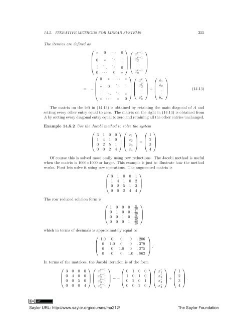
Page 357 and 358: 14.5. ITERATIVE METHODS FOR LINEAR
Page 359 and 360: 14.5. ITERATIVE METHODS FOR LINEAR
Page 361 and 362: 14.6. THEORY OF CONVERGENCE 361 Lem
Page 363 and 364: 14.7. EXERCISES 363 Proof: From Lem
Page 365 and 366: 14.7. EXERCISES 365 11. Suppose ρ
Page 367 and 368: 14.7. EXERCISES 367 Next take e tλ
Page 369 and 370: 14.7. EXERCISES 369 24. Suppose A i
Page 371 and 372: Numerical Methods For Finding Eigen
Page 373 and 374: 15.1. THE POWER METHOD FOR EIGENVAL
Page 387 and 388: 15.2. THE QR ALGORITHM 387 each a v
Page 389 and 390: 15.2. THE QR ALGORITHM 389 Proof: L
Page 391 and 392: 15.2. THE QR ALGORITHM 391 where
Page 393 and 394: 15.2. THE QR ALGORITHM 393 Corollar
Page 395 and 396: 15.2. THE QR ALGORITHM 395 below th
Page 397 and 398: 15.2. THE QR ALGORITHM 397 where R
Page 399 and 400: 15.2. THE QR ALGORITHM 399 A matrix
Page 401 and 402: 15.3. EXERCISES 401 where A k = Q k
Page 403 and 404: Positive Matrices Earlier theorems
Page 405 and 406:
405 |μ| ≤λ 0 . But also, the fa
Page 407 and 408:
407 which says x 0 −x 0 v T x 0 =
Page 409 and 410:
409 must have the same argument for
Page 411 and 412:
Functions Of Matrices The existence
Page 413 and 414:
413 There is no convergence problem
Page 415 and 416:
415 This gives us a nice definition
Page 417 and 418:
Applications To Differential Equati
Page 419 and 420:
C.3. LOCAL SOLUTIONS 419 C.3 Local
Page 421 and 422:
C.4. FIRST ORDER LINEAR SYSTEMS 421
Page 423 and 424:
Page 425 and 426:
Page 427 and 428:
Page 429 and 430:
C.5. GEOMETRIC THEORY OF AUTONOMOUS
Page 431 and 432:
C.5. GEOMETRIC THEORY OF AUTONOMOUS
Page 433 and 434:
C.6. GENERAL GEOMETRIC THEORY 433 T
Page 435 and 436:
C.7. THESTABLEMANIFOLD 435 Lemma C.
Page 437 and 438:
C.7. THESTABLEMANIFOLD 437 ≤ e γ
Page 439 and 440:
Compactness And Completeness D.0.1
Page 441 and 442:
441 |a k − a l | < ε 2 .Thenifk>
Page 443 and 444:
The Fundamental Theorem Of Algebra
Page 445 and 446:
Fields And Field Extensions F.1 The
Page 447 and 448:
F.2. THE FUNDAMENTAL THEOREM OF ALG
Page 449 and 450:
F.2. THE FUNDAMENTAL THEOREM OF ALG
Page 451 and 452:
F.3. TRANSCENDENTAL NUMBERS 451 F.3
Page 453 and 454:
F.3. TRANSCENDENTAL NUMBERS 453 It
Page 455 and 456:
F.3. TRANSCENDENTAL NUMBERS 455 Not
Page 457 and 458:
F.3. TRANSCENDENTAL NUMBERS 457 Thi
Page 459 and 460:
F.4. MORE ON ALGEBRAIC FIELD EXTENS
Page 461 and 462:
Page 463 and 464:
Page 465 and 466:
F.5. THE GALOIS GROUP 465 a rationa
Page 467 and 468:
F.5. THE GALOIS GROUP 467 Now let
Page 469 and 470:
F.6. NORMAL SUBGROUPS 469 If H is a
Page 471 and 472:
F.8. CONDITIONS FOR SEPARABILITY 47
Page 473 and 474:
F.8. CONDITIONS FOR SEPARABILITY 47
Page 475 and 476:
F.9. PERMUTATIONS 475 of f (x) ands
Page 477 and 478:
F.9. PERMUTATIONS 477 smallest k
Page 479 and 480:
F.10. SOLVABLE GROUPS 479 Then i 1
Page 481 and 482:
F.10. SOLVABLE GROUPS 481 Thus ever
Page 483 and 484:
F.11. SOLVABILITY BY RADICALS 483 A
Page 485 and 486:
Bibliography [1] Apostol T., Calcul
Page 487 and 488:
Answers To Selected Exercises G.1 E
Page 489 and 490:
G.7. EXERCISES 489 15 Find the matr
Page 491 and 492:
G.10. EXERCISES 491 11 It follows f
Page 493 and 494:
G.13. EXERCISES 493 19 ⎛ ⎝ 4
Page 495 and 496:
G.19. EXERCISES 495 8 λ 3 − λ 2
Page 497 and 498:
G.23. EXERCISES 497 ⎧⎛ ⎞⎫
Page 499 and 500:
INDEX 499 defective, 162 DeMoivre i
Page 501 and 502:
INDEX 501 rotation, 235 linear tran
Page 503:
INDEX 503 scalars, 18, 32, 37 Schur
show all

Linear Algebra, Theory And Applications, 2012a

You also want an ePaper? Increase the reach of your titles

Delete template?

Save as template?