- Page 2 and 3:
INTRODUCTION TO Health Physics
- Page 4 and 5:
INTRODUCTION TO Health Physics Herm
- Page 6 and 7:
To my wife, Sylvia and to the memor
- Page 8 and 9:
CONTENTS Preface/ XI 1. Introductio
- Page 10 and 11:
Surface Contamination Limits/592 Wa
- Page 12 and 13:
PREFACE The practice of radiation s
- Page 14 and 15:
INTRODUCTION TO Health Physics
- Page 16 and 17:
INTRODUCTION 1 Health physics, radi
- Page 18 and 19:
REVIEW OF PHYSICAL PRINCIPLES MECHA
- Page 20 and 21:
REVIEW OF PHYSICAL PRINCIPLES 5 In
- Page 22 and 23:
and at v = 0.99 c, m = 9.11 × 10
- Page 24 and 25:
REVIEW OF PHYSICAL PRINCIPLES 9 Sub
- Page 26 and 27:
REVIEW OF PHYSICAL PRINCIPLES 11 Th
- Page 28 and 29:
REVIEW OF PHYSICAL PRINCIPLES 13 co
- Page 30 and 31:
REVIEW OF PHYSICAL PRINCIPLES 15 Th
- Page 32 and 33:
REVIEW OF PHYSICAL PRINCIPLES 17 (t
- Page 34 and 35:
Electrical Current: The Ampere REVI
- Page 36 and 37:
Solution REVIEW OF PHYSICAL PRINCIP
- Page 38 and 39:
REVIEW OF PHYSICAL PRINCIPLES 23 Ac
- Page 40 and 41:
V a b REVIEW OF PHYSICAL PRINCIPLES
- Page 42 and 43:
Elastic Collision REVIEW OF PHYSICA
- Page 44 and 45:
Force Time REVIEW OF PHYSICAL PRINC
- Page 46 and 47:
REVIEW OF PHYSICAL PRINCIPLES 31 5
- Page 48 and 49:
REVIEW OF PHYSICAL PRINCIPLES 33 Fi
- Page 50 and 51:
REVIEW OF PHYSICAL PRINCIPLES 35 In
- Page 52 and 53:
REVIEW OF PHYSICAL PRINCIPLES 37 Th
- Page 54 and 55:
or, in terms of the loss tangent,
- Page 56 and 57:
where Impedance t = time after clos
- Page 58 and 59:
REVIEW OF PHYSICAL PRINCIPLES 43 Th
- Page 60 and 61:
REVIEW OF PHYSICAL PRINCIPLES 45 A
- Page 62 and 63:
therefore, Matter Waves REVIEW OF P
- Page 64 and 65:
REVIEW OF PHYSICAL PRINCIPLES 49 Th
- Page 66 and 67:
SUMMARY REVIEW OF PHYSICAL PRINCIPL
- Page 68 and 69:
REVIEW OF PHYSICAL PRINCIPLES 53 Ac
- Page 70 and 71:
REVIEW OF PHYSICAL PRINCIPLES 55 2.
- Page 72 and 73:
REVIEW OF PHYSICAL PRINCIPLES 57 2.
- Page 74 and 75:
ATOMIC AND NUCLEAR STRUCTURE ATOMIC
- Page 76 and 77:
Bohr’s Atomic Model ATOMIC AND NU
- Page 78 and 79:
ATOMIC AND NUCLEAR STRUCTURE 63 2.
- Page 80 and 81:
The energy of this photon is E = hc
- Page 82 and 83:
ATOMIC AND NUCLEAR STRUCTURE 67 are
- Page 84 and 85:
ATOMIC AND NUCLEAR STRUCTURE 69 ene
- Page 86 and 87:
TABLE 3-1. Electronic Structure of
- Page 88 and 89:
ATOMIC AND NUCLEAR STRUCTURE 73 rad
- Page 90 and 91:
ATOMIC AND NUCLEAR STRUCTURE 75 spe
- Page 92 and 93:
ATOMIC AND NUCLEAR STRUCTURE 77 whe
- Page 94 and 95:
ATOMIC AND NUCLEAR STRUCTURE 79 neu
- Page 96 and 97:
SUMMARY ATOMIC AND NUCLEAR STRUCTUR
- Page 98 and 99:
ATOMIC AND NUCLEAR STRUCTURE 83 3.1
- Page 100 and 101:
R ADIATION SOURCES RADIOACTIVITY 4
- Page 102 and 103:
R ADIATION SOURCES 87 Figure 4-2. T
- Page 104 and 105:
R ADIATION SOURCES 89 Figure 4-3. R
- Page 106 and 107:
R ADIATION SOURCES 91 Figure 4-4. P
- Page 108 and 109:
Figure 4-7. Iodine-131 transformati
- Page 110 and 111:
R ADIATION SOURCES 95 Since positro
- Page 112 and 113:
R ADIATION SOURCES 97 level of high
- Page 114 and 115:
R ADIATION SOURCES 99 From the defi
- Page 116 and 117:
R ADIATION SOURCES 101 determined b
- Page 118 and 119:
R ADIATION SOURCES 103 sum of the l
- Page 120 and 121:
R ADIATION SOURCES 105 of activity
- Page 122 and 123:
Solution SA 14 10 226 × 1600 yea
- Page 124 and 125:
and the number of radioactive atoms
- Page 126 and 127:
W EXAMPLE 4.8 R ADIATION SOURCES 11
- Page 128 and 129:
TABLE 4-2. Neptunium Series (4n +1)
- Page 130 and 131:
TABLE 4-4. Actinium Series (4n +3)
- Page 132 and 133:
R ADIATION SOURCES 117 TABLE 4-6. A
- Page 134 and 135:
The integrand can be changed to the
- Page 136 and 137:
Figure 4-14. Secular equilibrium: B
- Page 138 and 139:
R ADIATION SOURCES 123 of the daugh
- Page 140 and 141:
R ADIATION SOURCES 125 By the use o
- Page 142 and 143:
Expanding and collecting terms, we
- Page 144 and 145:
R ADIATION SOURCES 129 Figure 4-17.
- Page 146 and 147:
Deflector Vacuum pump External deam
- Page 148 and 149:
Substituting the value of r from Eq
- Page 150 and 151:
R ADIATION SOURCES 135 before it is
- Page 152 and 153:
R ADIATION SOURCES 137 4.18. What w
- Page 154 and 155:
R ADIATION SOURCES 139 4.43. 100-mC
- Page 156 and 157:
R ADIATION SOURCES 141 Report No. 1
- Page 158 and 159:
INTERACTION OF RADIATION WITH MATTE
- Page 160 and 161:
INTERACTION OF RADIATION WITH M ATT
- Page 162 and 163:
INTERACTION OF RADIATION WITH M ATT
- Page 164 and 165:
INTERACTION OF RADIATION WITH M ATT
- Page 166 and 167:
INTERACTION OF RADIATION WITH M ATT
- Page 168 and 169:
INTERACTION OF RADIATION WITH M ATT
- Page 170 and 171:
TABLE 5-2. Bremsstrahlung Spectrum
- Page 172 and 173:
INTERACTION OF RADIATION WITH M ATT
- Page 174 and 175:
INTERACTION OF RADIATION WITH M ATT
- Page 176 and 177:
INTERACTION OF RADIATION WITH M ATT
- Page 178 and 179:
INTERACTION OF RADIATION WITH M ATT
- Page 180 and 181:
INTERACTION OF RADIATION WITH M ATT
- Page 182 and 183:
INTERACTION OF RADIATION WITH M ATT
- Page 184 and 185:
INTERACTION OF RADIATION WITH M ATT
- Page 186 and 187:
W EXAMPLE 5.12 INTERACTION OF RADIA
- Page 188 and 189:
INTERACTION OF RADIATION WITH M ATT
- Page 190 and 191:
INTERACTION OF RADIATION WITH M ATT
- Page 192 and 193:
INTERACTION OF RADIATION WITH M ATT
- Page 194 and 195:
INTERACTION OF RADIATION WITH M ATT
- Page 196 and 197:
INTERACTION OF RADIATION WITH M ATT
- Page 198 and 199:
INTERACTION OF RADIATION WITH M ATT
- Page 200 and 201:
Classification TABLE 5-6. α, n Neu
- Page 202 and 203:
W EXAMPLE 5.14 INTERACTION OF RADIA
- Page 204 and 205:
since ln E =−ξ, E 0 E E 0 = e
- Page 206 and 207:
INTERACTION OF RADIATION WITH M ATT
- Page 208 and 209:
where INTERACTION OF RADIATION WITH
- Page 210 and 211:
INTERACTION OF RADIATION WITH M ATT
- Page 212 and 213:
INTERACTION OF RADIATION WITH M ATT
- Page 214 and 215:
INTERACTION OF RADIATION WITH M ATT
- Page 216 and 217:
INTERACTION OF RADIATION WITH M ATT
- Page 218 and 219:
UNITS RADIATION DOSIMETRY 6 During
- Page 220 and 221:
Solution The radiation absorbed dos
- Page 222 and 223:
RADIATION DOSIMETRY 207 The relatio
- Page 224 and 225:
RADIATION DOSIMETRY 209 The use of
- Page 226 and 227:
RADIATION DOSIMETRY 211 Since one e
- Page 228 and 229:
RADIATION DOSIMETRY 213 Figure 6-5.
- Page 230 and 231:
The radiation absorbed dose rate fr
- Page 232 and 233:
RADIATION DOSIMETRY 217 Figure 6-6.
- Page 234 and 235:
219 TABLE 6-1. Mean Mass Stopping P
- Page 236 and 237:
RADIATION DOSIMETRY 221 The exposur
- Page 238 and 239:
W Example 6.9 RADIATION DOSIMETRY 2
- Page 240 and 241:
RADIATION DOSIMETRY 225 This calcul
- Page 242 and 243:
where ϕ = intensity at depth t, ϕ
- Page 244 and 245:
RADIATION DOSIMETRY 229 Assuming th
- Page 246 and 247:
When we combine the constants in Eq
- Page 248 and 249:
Solution RADIATION DOSIMETRY 233 Ph
- Page 250 and 251:
RADIATION DOSIMETRY 235 In most ins
- Page 252 and 253:
RADIATION DOSIMETRY 237 first-order
- Page 254 and 255:
RADIATION DOSIMETRY 239 Integrating
- Page 256 and 257:
Medical Internal Radiation Dose Met
- Page 258 and 259:
RADIATION DOSIMETRY 243 1 Bq/cm 3 o
- Page 260 and 261:
W Example 6.16 RADIATION DOSIMETRY
- Page 262 and 263:
for 131I listed in the output data
- Page 264 and 265:
then the total dose to the target o
- Page 266 and 267:
251 TABLE 6-8. Absorbed Fractions (
- Page 268 and 269:
RADIATION DOSIMETRY 253 which was f
- Page 270 and 271:
255 TABLE 6-9. S, Absorbed Dose per
- Page 272 and 273:
257 TABLE 6-10. S, Absorbed Dose Pe
- Page 274 and 275:
RADIATION DOSIMETRY 259 values of S
- Page 276 and 277:
RADIATION DOSIMETRY 261 S (kidney
- Page 278 and 279:
RADIATION DOSIMETRY 263 and MIRD Pa
- Page 280 and 281:
RADIATION DOSIMETRY 265 the 50-year
- Page 282 and 283:
TABLE 6-11. Synthetic Tissue Compos
- Page 284 and 285:
Solution Dn,p = The dose rate due t
- Page 286 and 287:
RADIATION DOSIMETRY 271 6.2. An air
- Page 288 and 289:
RADIATION DOSIMETRY 273 (a) Plot th
- Page 290 and 291:
RADIATION DOSIMETRY 275 the averag
- Page 292 and 293:
RADIATION DOSIMETRY 277 No. 7. Berg
- Page 294 and 295:
7 BIOLOGICAL BASIS FOR RADIATION SA
- Page 296 and 297:
BIOLOGICAL BASIS FOR R ADIATION SAF
- Page 298 and 299:
BIOLOGICAL BASIS FOR R ADIATION SAF
- Page 300 and 301:
BIOLOGICAL BASIS FOR R ADIATION SAF
- Page 302 and 303:
Na + K + BIOLOGICAL BASIS FOR R ADI
- Page 304 and 305:
BIOLOGICAL BASIS FOR R ADIATION SAF
- Page 306 and 307:
BIOLOGICAL BASIS FOR R ADIATION SAF
- Page 308 and 309:
BIOLOGICAL BASIS FOR R ADIATION SAF
- Page 310 and 311:
TLC VC IC FRC IRV TV RV RV BIOLOGIC
- Page 312 and 313:
BIOLOGICAL BASIS FOR R ADIATION SAF
- Page 314 and 315:
Capillary knot Vein BIOLOGICAL BASI
- Page 316 and 317:
Cell body One nerve cell Axon Nucle
- Page 318 and 319:
BIOLOGICAL BASIS FOR R ADIATION SAF
- Page 320 and 321:
Aqueous humor Cornea Iris Lens Vitr
- Page 322 and 323:
BIOLOGICAL BASIS FOR R ADIATION SAF
- Page 324 and 325:
Leucocytes and lymphocytes (x10 −
- Page 326 and 327:
TABLE 7-5. Tissue Dose Rate vs. Dis
- Page 328 and 329:
Birth Defects (Teratogenesis) BIOLO
- Page 330 and 331:
BIOLOGICAL BASIS FOR R ADIATION SAF
- Page 332 and 333:
Cancer BIOLOGICAL BASIS FOR R ADIAT
- Page 334 and 335:
BIOLOGICAL BASIS FOR R ADIATION SAF
- Page 336 and 337:
BIOLOGICAL BASIS FOR R ADIATION SAF
- Page 338 and 339:
Incidence Incidence General form Do
- Page 340 and 341:
BIOLOGICAL BASIS FOR R ADIATION SAF
- Page 342 and 343:
BIOLOGICAL BASIS FOR R ADIATION SAF
- Page 344 and 345:
BIOLOGICAL BASIS FOR R ADIATION SAF
- Page 346 and 347:
BIOLOGICAL BASIS FOR R ADIATION SAF
- Page 348 and 349:
BIOLOGICAL BASIS FOR R ADIATION SAF
- Page 350 and 351:
BIOLOGICAL BASIS FOR R ADIATION SAF
- Page 352 and 353:
RADIATION SAFETY GUIDES 8 Radiation
- Page 354 and 355:
RADIATION SAFETY GUIDES 339 radiati
- Page 356 and 357:
RADIATION SAFETY GUIDES 341 members
- Page 358 and 359:
RADIATION SAFETY GUIDES 343 is a me
- Page 360 and 361:
RADIATION SAFETY GUIDES 345 Figure
- Page 362 and 363:
RADIATION SAFETY GUIDES 347 by radi
- Page 364 and 365:
RADIATION SAFETY GUIDES 349 radiati
- Page 366 and 367:
Dose Coefficient RADIATION SAFETY G
- Page 368 and 369:
RADIATION SAFETY GUIDES 353 appropr
- Page 370 and 371:
RADIATION SAFETY GUIDES 355 The cal
- Page 372 and 373:
Airborne Radioactivity RADIATION SA
- Page 374 and 375:
RADIATION SAFETY GUIDES 359 collisi
- Page 376 and 377:
RADIATION SAFETY GUIDES 361 is 1 g/
- Page 378 and 379:
RADIATION SAFETY GUIDES 363 Figure
- Page 380 and 381:
RADIATION SAFETY GUIDES 365 can be
- Page 382 and 383:
RADIATION SAFETY GUIDES 367 total w
- Page 384 and 385:
RADIATION SAFETY GUIDES 369 TABLE 8
- Page 386 and 387:
compartment after a time t is given
- Page 388 and 389:
RADIATION SAFETY GUIDES 373 Now we
- Page 390 and 391:
RADIATION SAFETY GUIDES 375 classi
- Page 392 and 393:
RADIATION SAFETY GUIDES 377 normal
- Page 394 and 395:
RADIATION SAFETY GUIDES 379 Figure
- Page 396 and 397:
RADIATION SAFETY GUIDES 381 whose c
- Page 398 and 399:
13 14 12 11 GI Tract 13 T RADIATION
- Page 400 and 401:
RADIATION SAFETY GUIDES 385 Figure
- Page 402 and 403:
RADIATION SAFETY GUIDES 387 REGION
- Page 404 and 405:
RADIATION SAFETY GUIDES 389 The bb
- Page 406 and 407:
391 TABLE 8-18. Values of Absorbed
- Page 408 and 409:
TABLE 8-19. Summary of Dose Calcula
- Page 410 and 411:
TABLE 8-20. Dose Coefficients for S
- Page 412 and 413:
RADIATION SAFETY GUIDES 397 nation
- Page 414 and 415:
and the total activity in the body
- Page 416 and 417:
RADIATION SAFETY GUIDES 401 segment
- Page 418 and 419:
RADIATION SAFETY GUIDES 403 where E
- Page 420 and 421:
TABLE 8-22. Radioisotopes That Do N
- Page 422 and 423:
RADIATION SAFETY GUIDES 407 The sma
- Page 424 and 425:
RADIATION SAFETY GUIDES 409 TABLE 8
- Page 426 and 427:
RADIATION SAFETY GUIDES 411 Kentuck
- Page 428 and 429:
RADIATION SAFETY GUIDES 413 The fra
- Page 430 and 431:
RADIATION SAFETY GUIDES 415 ALI = 1
- Page 432 and 433:
W Example 8.10 RADIATION SAFETY GUI
- Page 434 and 435:
W Example 8.12 RADIATION SAFETY GUI
- Page 436 and 437:
RADIATION SAFETY GUIDES 421 Substit
- Page 438 and 439:
RADIATION SAFETY GUIDES 423 64. Inf
- Page 440 and 441:
RADIATION SAFETY GUIDES 425 16. Pro
- Page 442 and 443:
HEALTH PHYSICS INSTRUMENTATION RADI
- Page 444 and 445:
Gas-Filled Particle Counters HEALTH
- Page 446 and 447:
HEALTH PHYSICS INSTRUMENTATION 431
- Page 448 and 449:
HEALTH PHYSICS INSTRUMENTATION 433
- Page 450 and 451:
HEALTH PHYSICS INSTRUMENTATION 435
- Page 452 and 453:
TABLE 9-2. Scintillating Materials
- Page 454 and 455: HEALTH PHYSICS INSTRUMENTATION 439
- Page 456 and 457: Figure 9-10. Block diagram of a sin
- Page 458 and 459: HEALTH PHYSICS INSTRUMENTATION 443
- Page 460 and 461: HEALTH PHYSICS INSTRUMENTATION 445
- Page 462 and 463: DOSE-MEASURING INSTRUMENTS HEALTH P
- Page 464 and 465: Response Normalized to Cs-137 10 Co
- Page 466 and 467: HEALTH PHYSICS INSTRUMENTATION 451
- Page 468 and 469: HEALTH PHYSICS INSTRUMENTATION 453
- Page 470 and 471: HEALTH PHYSICS INSTRUMENTATION 455
- Page 472 and 473: HEALTH PHYSICS INSTRUMENTATION 457
- Page 474 and 475: HEALTH PHYSICS INSTRUMENTATION 459
- Page 476 and 477: Survey Meters: Ion Current Chambers
- Page 478 and 479: W Example 9.6 HEALTH PHYSICS INSTRU
- Page 480 and 481: NEUTRON MEASUREMENTS HEALTH PHYSICS
- Page 482 and 483: 467 TABLE 9-4. Threshold Foil React
- Page 484 and 485: HEALTH PHYSICS INSTRUMENTATION 469
- Page 486 and 487: HEALTH PHYSICS INSTRUMENTATION 471
- Page 488 and 489: HEALTH PHYSICS INSTRUMENTATION 473
- Page 490 and 491: Count rate per unit flux 10 1 .1 .0
- Page 492 and 493: HEALTH PHYSICS INSTRUMENTATION 477
- Page 494 and 495: Solution HEALTH PHYSICS INSTRUMENTA
- Page 496 and 497: Neutrons TABLE 9-7. Calibration Sou
- Page 498 and 499: HEALTH PHYSICS INSTRUMENTATION 483
- Page 500 and 501: Accuracy HEALTH PHYSICS INSTRUMENTA
- Page 502 and 503: HEALTH PHYSICS INSTRUMENTATION 487
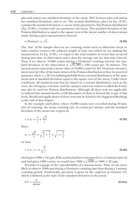
- Page 506 and 507: and is often expressed as a percent
- Page 508 and 509: HEALTH PHYSICS INSTRUMENTATION 493
- Page 510 and 511: HEALTH PHYSICS INSTRUMENTATION 495
- Page 512 and 513: HEALTH PHYSICS INSTRUMENTATION 497
- Page 514 and 515: W Example 9.16 What is the MDA for
- Page 516 and 517: Rearranging Eq. (9.60) and applying
- Page 518 and 519: For the data in this example: HEALT
- Page 520 and 521: Solution X = 1589 7 = 227 (Xi −
- Page 522 and 523: HEALTH PHYSICS INSTRUMENTATION 507
- Page 524 and 525: HEALTH PHYSICS INSTRUMENTATION 509
- Page 526 and 527: HEALTH PHYSICS INSTRUMENTATION 511
- Page 528 and 529: 10 EXTERNAL RADIATION SAFETY BASIC
- Page 530 and 531: EXTERNAL RADIATION SAFETY 515 By th
- Page 532 and 533: W Example 10.2 EXTERNAL RADIATION S
- Page 534 and 535: EXTERNAL RADIATION SAFETY 519 Figur
- Page 536 and 537: EXTERNAL RADIATION SAFETY 521 Figur
- Page 538 and 539: Au 198 Ir 192 Cs 137 EXTERNAL RADIA
- Page 540 and 541: Dose buildup factor, B Dose buildup
- Page 542 and 543: EXTERNAL RADIATION SAFETY 527 layer
- Page 544 and 545: X-Rays EXTERNAL RADIATION SAFETY 52
- Page 546 and 547: EXTERNAL RADIATION SAFETY 531 recom
- Page 548 and 549: where EXTERNAL RADIATION SAFETY 533
- Page 550 and 551: 535 TABLE 10-4. Values for the Para
- Page 552 and 553: EXTERNAL RADIATION SAFETY 537 a sec
- Page 554 and 555:
EXTERNAL RADIATION SAFETY 539 Figur
- Page 556 and 557:
TABLE 10-6. Commercial Lead Sheets
- Page 558 and 559:
EXTERNAL RADIATION SAFETY 543 The o
- Page 560 and 561:
EXTERNAL RADIATION SAFETY 545 Dist
- Page 562 and 563:
EXTERNAL RADIATION SAFETY 547 by th
- Page 564 and 565:
from Eqs. (10.26a) and (10.26b) int
- Page 566 and 567:
EXTERNAL RADIATION SAFETY 551 TABLE
- Page 568 and 569:
Transmission 1.0 86 4 2 10 8 6 4 -1
- Page 570 and 571:
EXTERNAL RADIATION SAFETY 555 to 0.
- Page 572 and 573:
The required lead-equivalent leaded
- Page 574 and 575:
Wpri = primary barrier weekly workl
- Page 576 and 577:
where EXTERNAL RADIATION SAFETY 561
- Page 578 and 579:
W = workload, Gy/wk, T = occupancy
- Page 580 and 581:
EXTERNAL RADIATION SAFETY 565 Gamm
- Page 582 and 583:
where Ni = number of atoms of the i
- Page 584 and 585:
EXTERNAL RADIATION SAFETY 569 which
- Page 586 and 587:
EXTERNAL RADIATION SAFETY 571 is fo
- Page 588 and 589:
where C = cost per unit volume of t
- Page 590 and 591:
EXTERNAL RADIATION SAFETY 575 for a
- Page 592 and 593:
EXTERNAL RADIATION SAFETY 577 Calcu
- Page 594 and 595:
EXTERNAL RADIATION SAFETY 579 per
- Page 596 and 597:
EXTERNAL RADIATION SAFETY 581 Patte
- Page 598 and 599:
11 INTERNAL R ADIATION SAFETY INTER
- Page 600 and 601:
INTERNAL RADIATION SAFETY 585 Figur
- Page 602 and 603:
INTERNAL RADIATION SAFETY 587 Figur
- Page 604 and 605:
INTERNAL RADIATION SAFETY 589 regar
- Page 606 and 607:
591 TABLE 11-3. Protection Factors
- Page 608 and 609:
INTERNAL RADIATION SAFETY 593 the m
- Page 610 and 611:
INTERNAL RADIATION SAFETY 595 TABLE
- Page 612 and 613:
INTERNAL RADIATION SAFETY 597 the U
- Page 614 and 615:
INTERNAL RADIATION SAFETY 599 Figur
- Page 616 and 617:
INTERNAL RADIATION SAFETY 601 effec
- Page 618 and 619:
603 TABLE 11-7. Treatment Methods f
- Page 620 and 621:
INTERNAL RADIATION SAFETY 605 or ba
- Page 622 and 623:
INTERNAL RADIATION SAFETY 607 Figur
- Page 624 and 625:
Figure 11-5. Gaussian plume dispers
- Page 626 and 627:
TABLE 11-10. Pasquill’s Categorie
- Page 628 and 629:
INTERNAL RADIATION SAFETY 613 is 4
- Page 630 and 631:
INTERNAL RADIATION SAFETY 615 Equat
- Page 632 and 633:
INTERNAL RADIATION SAFETY 617 In ce
- Page 634 and 635:
INTERNAL RADIATION SAFETY 619 In th
- Page 636 and 637:
INTERNAL RADIATION SAFETY 621 Since
- Page 638 and 639:
W Example 11.7 INTERNAL RADIATION S
- Page 640 and 641:
INTERNAL RADIATION SAFETY 625 In th
- Page 642 and 643:
INTERNAL RADIATION SAFETY 627 (b) A
- Page 644 and 645:
INTERNAL RADIATION SAFETY 629 a = c
- Page 646 and 647:
INTERNAL RADIATION SAFETY 631 treat
- Page 648 and 649:
INTERNAL RADIATION SAFETY 633 activ
- Page 650 and 651:
INTERNAL RADIATION SAFETY 635 Cohen
- Page 652 and 653:
INTERNAL RADIATION SAFETY 637 Repor
- Page 654 and 655:
CRITICALITY CRITICALITY HAZARD 12 O
- Page 656 and 657:
Potential energy E11 E12Em 2r Dista
- Page 658 and 659:
Fission Products CRITICALITY 643 Th
- Page 660 and 661:
CRITICALITY A2 = 2.35 × 10 15 1.2
- Page 662 and 663:
and will cause “fast fission.”
- Page 664 and 665:
W Example 12.3 CRITICALITY 649 Calc
- Page 666 and 667:
CRITICALITY 651 Making the very rea
- Page 668 and 669:
TABLE 12-3. Delayed Neutrons from t
- Page 670 and 671:
Power level dt t T τ then T = τ -
- Page 672 and 673:
CRITICALITY 657 TABLE 12-5. Activit
- Page 674 and 675:
TABLE 12-6. Minimum Critical Mass o
- Page 676 and 677:
SUMMARY CRITICALITY 661 a criticali
- Page 678 and 679:
CRITICALITY 663 12.10. The blood pl
- Page 680 and 681:
CRITICALITY 665 Knief, R. A. Nuclea
- Page 682 and 683:
EVALUATION OF RADIATION SAFETY MEAS
- Page 684 and 685:
Evaluation of Radiation Safety Meas
- Page 686 and 687:
Evaluation of Radiation Safety Meas
- Page 688 and 689:
Evaluation of Radiation Safety Meas
- Page 690 and 691:
Evaluation of Radiation Safety Meas
- Page 692 and 693:
Evaluation of Radiation Safety Meas
- Page 694 and 695:
W EXAMPLE 13.4 Evaluation of Radiat
- Page 696 and 697:
Evaluation of Radiation Safety Meas
- Page 698 and 699:
Evaluation of Radiation Safety Meas
- Page 700 and 701:
Evaluation of Radiation Safety Meas
- Page 702 and 703:
Evaluation of Radiation Safety Meas
- Page 704 and 705:
Evaluation of Radiation Safety Meas
- Page 706 and 707:
Evaluation of Radiation Safety Meas
- Page 708 and 709:
Evaluation of Radiation Safety Meas
- Page 710 and 711:
Evaluation of Radiation Safety Meas
- Page 712 and 713:
Evaluation of Radiation Safety Meas
- Page 714 and 715:
Evaluation of Radiation Safety Meas
- Page 716 and 717:
W EXAMPLE 13.9 Evaluation of Radiat
- Page 718 and 719:
Evaluation of Radiation Safety Meas
- Page 720 and 721:
Evaluation of Radiation Safety Meas
- Page 722 and 723:
Evaluation of Radiation Safety Meas
- Page 724 and 725:
SUMMARY Evaluation of Radiation Saf
- Page 726 and 727:
Evaluation of Radiation Safety Meas
- Page 728 and 729:
(b) Are the distributions normal or
- Page 730 and 731:
Evaluation of Radiation Safety Meas
- Page 732 and 733:
Evaluation of Radiation Safety Meas
- Page 734 and 735:
Evaluation of Radiation Safety Meas
- Page 736 and 737:
NONIONIZING RADIATION SAFETY 14 Non
- Page 738 and 739:
Solution NONIONIZING RADIATION SAFE
- Page 740 and 741:
NONIONIZING RADIATION SAFETY 725 hi
- Page 742 and 743:
2.4 mW cm 2 E mW cm 2 = (50 cm)2 (1
- Page 744 and 745:
NONIONIZING RADIATION SAFETY 729 Fi
- Page 746 and 747:
NONIONIZING RADIATION SAFETY 731 Fi
- Page 748 and 749:
Figure 14-4. Beam cross sections fo
- Page 750 and 751:
% Total Transmission 100 90 80 70 6
- Page 752 and 753:
NONIONIZING RADIATION SAFETY 737 TA
- Page 754 and 755:
NONIONIZING RADIATION SAFETY 739 TA
- Page 756 and 757:
NONIONIZING RADIATION SAFETY 741 TA
- Page 758 and 759:
W Example 14.7 NONIONIZING RADIATIO
- Page 760 and 761:
NONIONIZING RADIATION SAFETY 745 Th
- Page 762 and 763:
TABLE 14-12. Reflecting Materials N
- Page 764 and 765:
Solution NONIONIZING RADIATION SAFE
- Page 766 and 767:
Solution The irradiance at the aper
- Page 768 and 769:
Wavelengths (nm) NONIONIZING RADIAT
- Page 770 and 771:
n = 300 pulses s × 10 seconds = 30
- Page 772 and 773:
% of Peak 100 80 60 40 20 NONIONIZI
- Page 774 and 775:
NONIONIZING RADIATION SAFETY 759 Th
- Page 776 and 777:
TABLE 14-16. Radar Bands FREQUENCY
- Page 778 and 779:
NONIONIZING RADIATION SAFETY 763 Al
- Page 780 and 781:
NONIONIZING RADIATION SAFETY 765 po
- Page 782 and 783:
NONIONIZING RADIATION SAFETY 767 Gr
- Page 784 and 785:
NONIONIZING RADIATION SAFETY 769 in
- Page 786 and 787:
Since there is 1 J/s in a watt, 1.1
- Page 788 and 789:
NONIONIZING RADIATION SAFETY 773 Th
- Page 790 and 791:
Biological Effects NONIONIZING RADI
- Page 792 and 793:
where Td = dry bulb temperature,
- Page 794 and 795:
NONIONIZING RADIATION SAFETY 779 to
- Page 796 and 797:
NONIONIZING RADIATION SAFETY 781 th
- Page 798 and 799:
Dosimetry NONIONIZING RADIATION SAF
- Page 800 and 801:
NONIONIZING RADIATION SAFETY 785 Fi
- Page 802 and 803:
NONIONIZING RADIATION SAFETY 787 TA
- Page 804 and 805:
where S = power density, W/m 2 , ε
- Page 806 and 807:
NONIONIZING RADIATION SAFETY 791 ME
- Page 808 and 809:
where A = attenuation, dB, t = shie
- Page 810 and 811:
NONIONIZING RADIATION SAFETY 795 th
- Page 812 and 813:
NONIONIZING RADIATION SAFETY 797 14
- Page 814 and 815:
NONIONIZING RADIATION SAFETY 799 SO
- Page 816 and 817:
NONIONIZING RADIATION SAFETY 801 Ha
- Page 818 and 819:
APPENDIX A Values of Some Useful Co
- Page 820 and 821:
APPENDIX B Table of the Elements NA
- Page 822 and 823:
Table of the Elements (Continued) A
- Page 824 and 825:
APPENDIX C The Reference Person Ove
- Page 826 and 827:
Chemical Composition APPENDIX C. 81
- Page 828 and 829:
Duration of Exposure 1. Occupationa
- Page 830 and 831:
APPENDIX D SPECIFIC ABSORBED FRACTI
- Page 832 and 833:
817 Energy in (MeV) Target 0.200 0.
- Page 834 and 835:
819 Energy in (MeV) Target 0.200 0.
- Page 836 and 837:
821 Energy in (MeV) Target 0.200 0.
- Page 838 and 839:
823 Energy in (MeV) Target 0.200 0.
- Page 840 and 841:
825 Energy in (MeV) Target 0.200 0.
- Page 842 and 843:
827 Energy in (MeV) Target 0.200 0.
- Page 844 and 845:
829 Energy in (MeV) Target 0.200 0.
- Page 846 and 847:
831 Energy in (MeV) Target 0.200 0.
- Page 848 and 849:
833 Energy in (MeV) Target 0.200 0.
- Page 850 and 851:
835 Energy in (MeV) Target 0.200 0.
- Page 852 and 853:
837 Energy in (MeV) Target 0.200 0.
- Page 854 and 855:
839 Energy in (MeV) Target 0.200 0.
- Page 856 and 857:
841 Energy in (MeV) Target 0.200 0.
- Page 858 and 859:
843 Energy in (MeV) Target 0.200 0.
- Page 860 and 861:
845 Target 0.200 0.500 1.000 1.500
- Page 862 and 863:
847 Energy in (MeV) Target 0.200 0.
- Page 864 and 865:
849 Energy in (MeV) Target 0.200 0.
- Page 866 and 867:
APPENDIX E TOTAL MASS ATTENUATION C
- Page 868 and 869:
APPENDIX F MASS ENERGY ABSORPTION C
- Page 870 and 871:
ANSWERS TO PROBLEMS 2.1 0.53 m/s to
- Page 872 and 873:
TVL Al 5.3 cm 0.1 MeV Cu 0.6 cm
- Page 874 and 875:
12.2 Nuclide Bq/L pCi/mL 24 Na 1200
- Page 876 and 877:
INDEX Page numbers followed by “t
- Page 878 and 879:
Catecholamines, 303 Cavity ionizati
- Page 880 and 881:
Energy Research and Development Adm
- Page 882 and 883:
International Organization for Stan
- Page 884 and 885:
n-p junction, 445 Nuclear bombings
- Page 886 and 887:
Radium injections, 324 Radon daught
- Page 888:
Type 2, or non-insulin-dependent di