Carsten Timm: Theory of superconductivity
Carsten Timm: Theory of superconductivity
Carsten Timm: Theory of superconductivity

You also want an ePaper? Increase the reach of your titles
YUMPU automatically turns print PDFs into web optimized ePapers that Google loves.
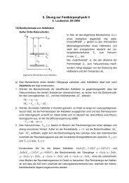
k y<br />
0<br />
Q<br />
k x<br />
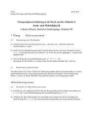
This type <strong>of</strong> gap is called a d x2 −y 2-wave (or just d-wave) gap since it has the symmetry <strong>of</strong> a d x 2 −y 2-orbital<br />
(though in k-space, not in real space). The simplest gap function with this symmetry and consistent with the<br />
lattice structure is<br />
∆ k = ∆ 0 (cos k x a − cos k y a). (12.8)<br />
Recall that the gap function away from the Fermi surface is <strong>of</strong> limited importance.<br />
The d-wave gap ∆ k is distinct from the conventional, approximately constant s-wave gap in that it has zeroes<br />
on the Fermi surface. These zeroes are called gap nodes. In the present case they appear in the (11) and equivalent<br />
directions. The quasiparticle dispersion in the vicinity <strong>of</strong> such a node is<br />
√<br />
E k =<br />
√ξk 2 + |∆ k| 2 ∼ = (ϵ k − µ) 2 + ∆ 2 0 (cos k xa − cos k y a) 2 . (12.9)<br />
One node is at<br />
k 0 = k ( )<br />
F 1<br />
√ . (12.10)<br />
2 1<br />
Writing k = k 0 + q and expanding for small q, we obtain<br />
E ∼ √<br />
k0+q = (v F · q) 2 + ∆ 2 0 [−(sin k0 xa)q x a + (sin kya)q 0 y a] 2 , (12.11)<br />
where<br />
v F := ∂ϵ k<br />
∂k<br />
∣<br />
∣<br />
k=k0<br />
= v ( )<br />
F 1<br />
√<br />
2 1<br />
(12.12)<br />
is the normal-state Fermi velocity at the node. Thus<br />
√<br />
[(<br />
E ∼ k0 +q = (v F · q) 2 + ∆ 2 0 −a sin k F a<br />
√ , a sin k ) 2 √<br />
F a<br />
√ · q]<br />
= (v F · q) 2 + (v qp · q) 2 , (12.13)<br />
2 2<br />
where<br />
v qp := ∆ 0 a sin k ( )<br />
F a −1<br />
√ ⊥ v 2 1<br />
F . (12.14)<br />
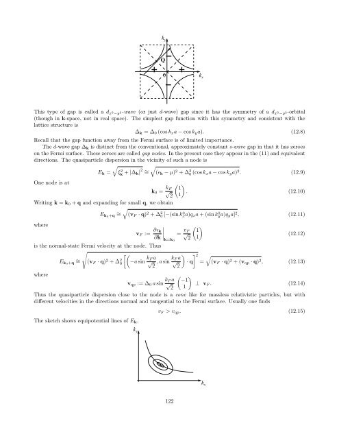
Thus the quasiparticle dispersion close to the node is a cone like for massless relativistic particles, but with<br />
different velocities in the directions normal and tangential to the Fermi surface. Usually one finds<br />
The sketch shows equipotential lines <strong>of</strong> E k .<br />
k y<br />
v F > v qp . (12.15)<br />
k x<br />
122