Carsten Timm: Theory of superconductivity

Since all coefficients are real, the solution can be chosen real. For x → ∞ we should obtain the uniform solution
√
lim ψ(x) = − α
x→∞ β . (6.22)
Writing
ψ(x) =
√
− α f(x) (6.23)
β
we obtain
This equation contains a characteristic length ξ with
2
−
2m ∗ f ′′ (x) + f(x) − f(x) 3 = 0. (6.24)
} {{
α
}
> 0
ξ 2 = −
2
2m ∗ α ∼ 2
=
2m ∗ α ′ > 0, (6.25)
(T c − T )
which is called the Ginzburg-Landau coherence length. It is not the same quantity as the the Pippard coherence
length ξ 0 or ξ. The Ginzburg-Landau ξ has a strong temperature dependence and actually diverges at T = T c ,
whereas the Pippard ξ has at most a weak temperature dependence. Microscopic BCS theory reveals how the
two quantities are related, though. Equation (6.24) can be solved analytically. It is easy to check that
f(x) = tanh
x √
2 ξ
(6.26)
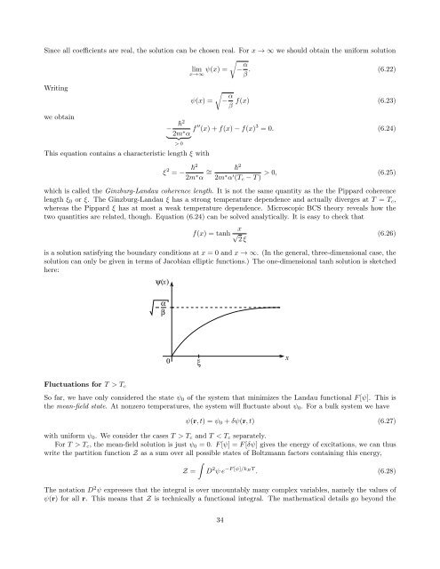
is a solution satisfying the boundary conditions at x = 0 and x → ∞. (In the general, three-dimensional case, the
solution can only be given in terms of Jacobian elliptic functions.) The one-dimensional tanh solution is sketched
here:
ψ(x)
α
β
0 ξ
x
Fluctuations for T > T c
So far, we have only considered the state ψ 0 of the system that minimizes the Landau functional F [ψ]. This is
the mean-field state. At nonzero temperatures, the system will fluctuate about ψ 0 . For a bulk system we have
ψ(r, t) = ψ 0 + δψ(r, t) (6.27)
with uniform ψ 0 . We consider the cases T > T c and T < T c separately.
For T > T c , the mean-field solution is just ψ 0 = 0. F [ψ] = F [δψ] gives the energy of excitations, we can thus
write the partition function Z as a sum over all possible states of Boltzmann factors containing this energy,
∫
Z = D 2 ψ e −F [ψ]/kBT . (6.28)
The notation D 2 ψ expresses that the integral is over uncountably many complex variables, namely the values of
ψ(r) for all r. This means that Z is technically a functional integral. The mathematical details go beyond the
34