Carsten Timm: Theory of superconductivity

Specifically, we have
G R (rσt, r ′ σ ′ t ′ ) =−i Θ(t − t ′ ) 1 Z Tr e−βH( e iHt/ Ψ σ (r) e −iH(t−t′ )/ Ψ † σ ′(r′ ) e −iHt′ /
+ e iHt′ / Ψ † σ ′(r′ ) e −iH(t′ −t)/ Ψ σ (r) e −iHt/) . (8.13)
In practice, we will want to write the Hamiltonian in the form H = H 0 + V and treat V in perturbation theory.
It is not surprising that this is complicated due to the presence of H in several exponential factors. However,
these factors are of a similar form, only in some the prefactor of H is imaginary and in one it is the real inverse
temperature. Can one simplify calculations by making all prefactors real? This is indeed possible by formally
replacing t → −iτ, t ′ → −iτ ′ , which is the main idea behind the imaginary-time formalism. We cannot discuss
it here but only state a few relevant results.
It turns out to be useful to consider the Matsubara (or thermal) Green function
⟨
⟩
G(rσt, r ′ σ ′ t ′ ) := − T τ Ψ σ (r, t)Ψ † σ ′(r′ , t ′ ) , (8.14)
where for any operator
and T τ is a time-ordering directive:
T τ A(τ)B(τ ′ ) =
A(τ) := e Hτ/ A e −Hτ/ . (8.15)
{
A(τ)B(τ ′ ) for τ > τ ′
±B(τ ′ )A(τ) for τ < τ ′ (8.16)
(upper/lower sign for bosonic/fermionic operators). For time-independent Hamiltonians, the Green function only
depends on the difference τ − τ ′ . One can then show that the resulting Green function G(rσ, r ′ σ ′ , τ) is defined
only for τ ∈ [−β, β] and satisfies
G(rσ, r ′ σ ′ , τ + β) = −G(rσ, r ′ σ ′ , τ) (8.17)
for fermions. This implies that the Fourier transform is a discrete sum over the fermionic Matsubara frequencies
ω n :=
(2n + 1)π
, n ∈ Z. (8.18)
β
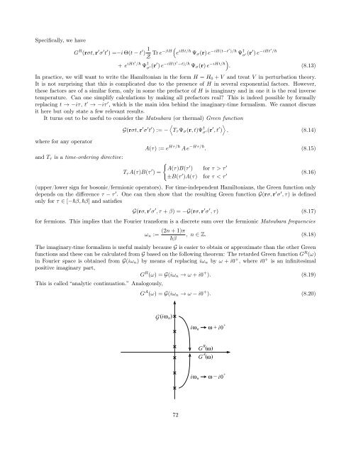
The imaginary-time formalism is useful mainly because G is easier to obtain or approximate than the other Green
functions and these can be calculated from G based on the following theorem: The retarded Green function G R (ω)
in Fourier space is obtained from G(iω n ) by means of replacing iω n by ω + i0 + , where i0 + is an infinitesimal
positive imaginary part,
G R (ω) = G(iω n → ω + i0 + ). (8.19)
This is called “analytic continuation.” Analogously,
G A (ω) = G(iω n → ω − i0 + ). (8.20)
G ( iω n )
ω n
i ω + i0 +
R
G (ω)
A
G (ω)
i ω − i0 +
ω n
72