Set of supplementary notes.

1.1. LORENTZ OSCILLATOR MODEL 11
Im(ε)
Permittivity ε
1
0
Re(ε)
0 ω Τ
Frequency
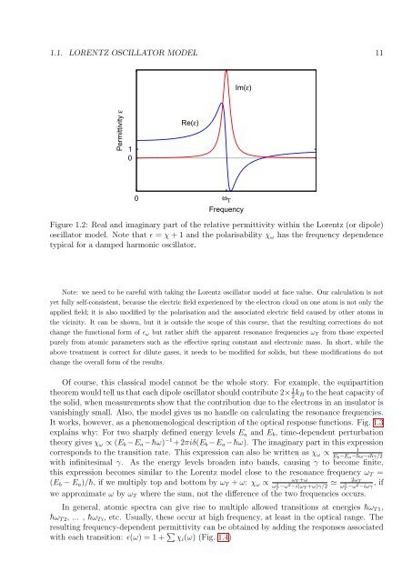
Figure 1.2: Real and imaginary part of the relative permittivity within the Lorentz (or dipole)
oscillator model. Note that ɛ = χ + 1 and the polarisability χ ω has the frequency dependence
typical for a damped harmonic oscillator.
Note: we need to be careful with taking the Lorentz oscillator model at face value. Our calculation is not
yet fully self-consistent, because the electric field experienced by the electron cloud on one atom is not only the
applied field; it is also modified by the polarisation and the associated electric field caused by other atoms in
the vicinity. It can be shown, but it is outside the scope of this course, that the resulting corrections do not
change the functional form of ɛ ω but rather shift the apparent resonance frequencies ω T from those expected
purely from atomic parameters such as the effective spring constant and electronic mass. In short, while the
above treatment is correct for dilute gases, it needs to be modified for solids, but these modifications do not
change the overall form of the results.
Of course, this classical model cannot be the whole story. For example, the equipartition
theorem would tell us that each dipole oscillator should contribute 2× 1k 2 B to the heat capacity of
the solid, when measurements show that the contribution due to the electrons in an insulator is
vanishingly small. Also, the model gives us no handle on calculating the resonance frequencies.
It works, however, as a phenomenological description of the optical response functions. Fig. 1.3
explains why: For two sharply defined energy levels E a and E b , time-dependent perturbation
theory gives χ ω ∝ (E b −E a −h¯ω) −1 +2πiδ(E b −E a −h¯ω). The imaginary part in this expression
1
corresponds to the transition rate. This expression can also be written as χ ω ∝
E b −E a−h¯ω−ih¯γ/2
with infinitesimal γ. As the energy levels broaden into bands, causing γ to become finite,
this expression becomes similar to the Lorentz model close to the resonance frequency ω T =
ω
(E b − E a )/h¯, if we multiply top and bottom by ω T + ω: χ ω ∝
T +ω
≃ 2ω T
, if
ωT 2 −ω2 −i(ω T +ω)γ/2 ωT 2 −ω2 −iωγ
we approximate ω by ω T where the sum, not the difference of the two frequencies occurs.
In general, atomic spectra can give rise to multiple allowed transitions at energies h¯ω T 1 ,
h¯ω T 2 , ... , h¯ω T i , etc. Usually, these occur at high frequency, at least in the optical range. The
resulting frequency-dependent permittivity can be obtained by adding the responses associated
with each transition: ɛ(ω) = 1 + ∑ χ i (ω) (Fig. 1.4)