Set of supplementary notes.

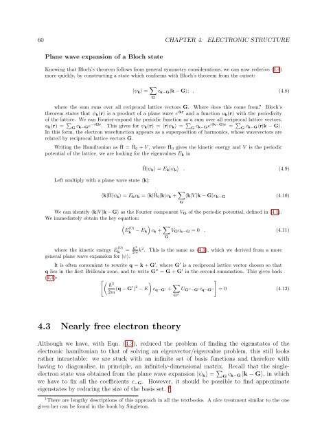
60 CHAPTER 4. ELECTRONIC STRUCTURE
Plane wave expansion of a Bloch state
Knowing that Bloch’s theorem follows from general symmetry considerations, we can now rederive (4.4)
more quickly, by constructing a state which conforms with Bloch’s theorem from the outset:
|ψ k 〉 = ∑ G
c k−G |k − G〉; , (4.8)
where the sum runs over all reciprocal lattice vectors G. Where does this come from Bloch’s
theorem states that ψ k (r) is a product of a plane wave e ikr and a function u k (r) with the periodicity
of the lattice. We can Fourier-expand the periodic function as a sum over all reciprocal lattice vectors,
u k (r) = ∑ G c k−Ge −iGr . This gives for ψ k (r) = 〈r|ψ k 〉 = ∑ G c k−Ge i(k−G)r = ∑ G c k−G〈r|k − G〉.
In this form, the electron wavefunction appears as a superposition of harmonics, whose wavevectors are
related by reciprocal lattice vectors G.
Writing the Hamiltonian as Ĥ = Ĥ0 + V , where Ĥ0 gives the kinetic energy and V is the periodic
potential of the lattice, we are looking for the eigenvalues E k in
Left multiply with a plane wave state 〈k|:
Ĥ|ψ k 〉 = E k |ψ k 〉 . (4.9)
〈k|Ĥ|ψ k〉 = E k c k = 〈k|Ĥ0|k〉c k + ∑ G
〈k|V |k − G〉c k−G (4.10)
We can identify 〈k|V |k − G〉 as the Fourier component V G of the periodic potential, defined in (4.1).
We immediately obtain the key equation:
( )
E (0)
k
− E k c k + ∑ V G c k−G = 0 , (4.11)
G
where the kinetic energy E (0)
k
= h¯ 2
2m k2 . This is the same as (4.3), which we derived from a more
general plane wave expansion for |ψ〉.
It is often convenient to rewrite q = k + G ′ , where G ′ is a reciprocal lattice vector chosen so that
q lies in the first Brillouin zone, and to write G ′′ = G + G ′ in the second summation. This gives back
(4.4): [ ( ) h¯2
2m (q − G′ ) 2 − E c q−G ′ + ∑ ]
U G ′′ −G ′c q−G ′′ = 0 (4.12)
G ′′
4.3 Nearly free electron theory
Although we have, with Eqn. (4.3), reduced the problem of finding the eigenstates of the
electronic hamiltonian to that of solving an eigenvector/eigenvalue problem, this still looks
rather intractable: we are stuck with an infinite set of basis functions and therefore with
having to diagonalise, in principle, an infinitely-dimensional matrix. Recall that the singleelectron
state was obtained from the plane wave expansion |ψ k 〉 = ∑ G c k−G |k − G〉, in which
we have to fix all the coefficients c −G . However, it should be possible to find approximate
eigenstates by reducing the size of the basis set. 1
1 There are lengthy descriptions of this approach in all the textbooks. A nice treatment similar to the one
given her can be found in the book by Singleton.