Set of supplementary notes.
Set of supplementary notes.
Set of supplementary notes.

You also want an ePaper? Increase the reach of your titles
YUMPU automatically turns print PDFs into web optimized ePapers that Google loves.
76 CHAPTER 5. BANDSTRUCTURE OF REAL MATERIALS<br />
• You will also <strong>of</strong>ten see particular bands labelled either along lines or at points by greek<br />
or latin capital letters with a subscript. These notations label the group representation<br />
<strong>of</strong> the state (symmetry) and we won’t discuss them further here.<br />
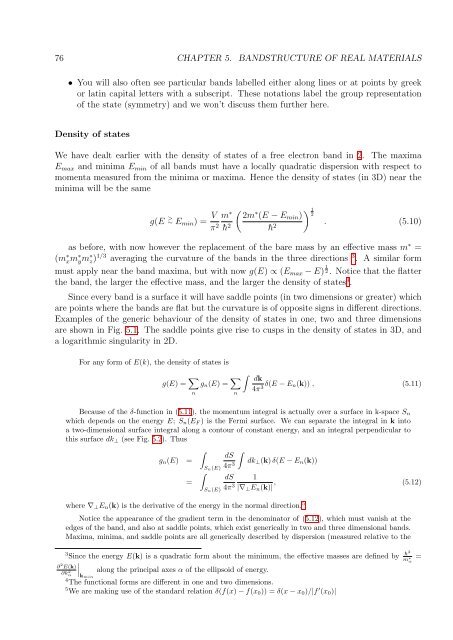
Density <strong>of</strong> states<br />
We have dealt earlier with the density <strong>of</strong> states <strong>of</strong> a free electron band in 2. The maxima<br />
E max and minima E min <strong>of</strong> all bands must have a locally quadratic dispersion with respect to<br />
momenta measured from the minima or maxima. Hence the density <strong>of</strong> states (in 3D) near the<br />
minima will be the same<br />
g(E > ∼ E min ) = V (<br />
m ∗ 2m ∗ (E − E min )<br />
π 2 h¯ 2 h¯ 2<br />
) 1<br />
2<br />
. (5.10)<br />
as before, with now however the replacement <strong>of</strong> the bare mass by an effective mass m ∗ =<br />
(m ∗ xm ∗ ym ∗ z) 1/3 averaging the curvature <strong>of</strong> the bands in the three directions 3 . A similar form<br />
must apply near the band maxima, but with now g(E) ∝ (E max − E) 1 2 . Notice that the flatter<br />
the band, the larger the effective mass, and the larger the density <strong>of</strong> states 4 .<br />
Since every band is a surface it will have saddle points (in two dimensions or greater) which<br />
are points where the bands are flat but the curvature is <strong>of</strong> opposite signs in different directions.<br />
Examples <strong>of</strong> the generic behaviour <strong>of</strong> the density <strong>of</strong> states in one, two and three dimensions<br />
are shown in Fig. 5.1. The saddle points give rise to cusps in the density <strong>of</strong> states in 3D, and<br />
a logarithmic singularity in 2D.<br />
For any form <strong>of</strong> E(k), the density <strong>of</strong> states is<br />
g(E) = ∑ n<br />
g n (E) = ∑ n<br />
∫<br />
dk<br />
4π 3 δ(E − E n(k)) , (5.11)<br />
Because <strong>of</strong> the δ-function in (5.11), the momentum integral is actually over a surface in k-space S n<br />
which depends on the energy E; S n (E F ) is the Fermi surface. We can separate the integral in k into<br />
a two-dimensional surface integral along a contour <strong>of</strong> constant energy, and an integral perpendicular to<br />
this surface dk ⊥ (see Fig. 5.2). Thus<br />
g n (E) =<br />
=<br />
∫<br />
∫<br />
S n(E)<br />
S n(E)<br />
∫<br />
dS<br />
4π 3<br />
dk ⊥ (k) δ(E − E n (k))<br />
where ∇ ⊥ E n (k) is the derivative <strong>of</strong> the energy in the normal direction. 5<br />
dS<br />
4π 3 1<br />
|∇ ⊥ E n (k)| , (5.12)<br />
Notice the appearance <strong>of</strong> the gradient term in the denominator <strong>of</strong> (5.12), which must vanish at the<br />
edges <strong>of</strong> the band, and also at saddle points, which exist generically in two and three dimensional bands.<br />
Maxima, minima, and saddle points are all generically described by dispersion (measured relative to the<br />
3 Since the energy E(k) is a quadratic form about the minimum, the effective masses are defined by h¯ 2<br />
m ∗ α<br />
∣<br />
along the principal axes α <strong>of</strong> the ellipsoid <strong>of</strong> energy.<br />
∂ 2 E(k)<br />
∂k<br />
∣<br />
α<br />
2 kmin<br />
4 The functional forms are different in one and two dimensions.<br />
5 We are making use <strong>of</strong> the standard relation δ(f(x) − f(x 0 )) = δ(x − x 0 )/|f ′ (x 0 )|<br />
=