Set of supplementary notes.

More documents

Recommendations

Info

26 CHAPTER 2. SOMMERFELD THEORY 2.4 Thermal properties of the electron gas The occupancy of states in thermal equilibrium in a fermi system is governed by the fermi distribution 1 f(E) = (2.12) e (E−µ)/k BT + 1 where the chemical potential µ can be identified (at zero temperature) with the fermi energy E F of the previous section. The number density of particles is n = N/V = 1 ∑ f(E i ) = 2 ∑ f(ɛ k ) V V i k = 1 ∫ dkf(ɛ 4π 3 k ) ∫ = dE g(E)f(E) (2.13) The internal energy density u = U/V can then be written in the same fashion: ∫ u = dE Eg(E)f(E) (2.14) (2.14) will be used to derive the electronic specific heat c v = ∂u/∂T | v at constant volume. The estimation is made much simpler by realising that in almost all cases of interest, the energy scale set by temperature k B T (≈ 0.025 eV at room temperature) is much less than the fermi energy E F (a few eV in most metals). From (2.14) ∫ c v = dE Eg(E) ∂f(E) ∂T (2.15) Notice that the fermi function is very nearly a step-function, so that the temperature-derivative is a function that is sharply-peaked for energies near the chemical potential. The contribution to the specific heat then comes only from states within k B T of the chemical potential and is much less than the 3/2k B per particle from classical distinguishable particles. From such an argument, one guesses that the specific heat per unit volume is of order c v ≈ N V k B T E F k B (2.16) Doing the algebra is a little tricky, because it is important to keep the number density fixed ((2.13)) — which requires the chemical potential to shift (a little) with temperature since the density of states is not constant. A careful calculation is given by Ashcroft and Mermin. But to the extent that we can take the density of states to be a constant, we can remove the factors g(E) from inside the integrals. Notice that with the change of variable x = (E − µ)/k B T df dT = e x (e x + 1) 2 × [ x T + 1 k B T ] dµ dT (2.17)
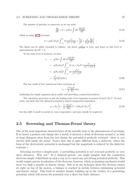
2.5. SCREENING AND THOMAS-FERMI THEORY 27 The number of particles is conserved, so we can write ∫ dn dT = 0 = g(E F ) dE ∂f(E) ∂T which on using (2.17) becomes 0 = g(E F )k B T ∫ ∞ −∞ The limits can be safely extended to infinity: the factor approximation dµ/dT = 0. To the same level of accuracy, we have ∫ c v = g(E F ) dE E ∂f(E) ∂T = g(E F )k B T = g(E F )k 2 BT e x [ x dx (e x + 1) 2 × T + 1 ] dµ k B T dT ∫ ∞ −∞ ∫ ∞ −∞ The last result is best understood when rewritten as (2.18) . (2.19) e x (e x +1) 2 is even, and hence at this level of e x x dx (µ + k B T x) (e x + 1) 2 T dx x 2 e x (e x + 1) 2 = π2 3 k2 BT g(E F ) (2.20) c v = π2 2 k B T E F nk B (2.21) confirming the simple argument given earlier and providing a numerical prefactor. The calculation given here is just the leading order of an expansion in powers of (k B T/E F ) 2 . To next order, one finds that the chemical potential is indeed temperature-dependent: [ µ = E F 1 − 1 ] 3 (πk BT ) 2 + O(k B T/E F ) 4 (2.22) 2E F but this shift is small in metals at room temperature, and may usually be neglected. 2.5 Screening and Thomas-Fermi theory One of the most important characteristics of the metallic state is the phenomenon of screening. If we insert a positive test charge into a metal, it attracts a cloud of electrons around it, so that at large distances away from the test charge the potential is perfectly screened - there is zero electric field inside the metal. Notice that this is quite different from a dielectric, where the form of the electrostatic potential is unchanged but the magnitude is reduced by the dielectric constant ɛ. Screening involves a length-scale: a perturbing potential is not screened perfectly at very short distances. Why not In a classical picture, one might imagine that the conduction electrons simply redistribute in such a way as to cancel any perturbing potential perfectly. This would require precise localisation of the electrons, however, which in quantum mechanics would incur too high a penalty in kinetic energy. Just as in the hydrogen atom the electron cannot sit right on top of the proton, a balance is reached in metals between minimising potential and kinetic energy. This leads to number density building up in the vicinity of a perturbing potential, which will screen the potential over a short but finite distance.
Page 1: Quantum Condensed Matter Physics Pa
Page 4 and 5: 4 CONTENTS 5.1 Bands and Brillouin
Page 6 and 7: 6 CONTENTS also serves to give impo
Page 8 and 9: 8 CONTENTS
Page 10 and 11: 10 CHAPTER 1. CLASSICAL MODELS FOR
Page 24 and 25: 24 CHAPTER 2. SOMMERFELD THEORY Fig
Page 28 and 29: 28 CHAPTER 2. SOMMERFELD THEORY Res
Page 30 and 31: 30 CHAPTER 2. SOMMERFELD THEORY Thi
Page 32 and 33: 32 CHAPTER 2. SOMMERFELD THEORY
Page 34 and 35: 34 CHAPTER 3. FROM ATOMS TO SOLIDS
Page 56 and 57: 56 CHAPTER 4. ELECTRONIC STRUCTURE
Page 74 and 75: 74 CHAPTER 5. BANDSTRUCTURE OF REAL
Page 76 and 77:
76 CHAPTER 5. BANDSTRUCTURE OF REAL
Page 78 and 79:
Page 80 and 81:
Page 82 and 83:
Page 84 and 85:
Page 86 and 87:
Page 88 and 89:
88 CHAPTER 6. EXPERIMENTAL PROBES O
Page 90 and 91:
Page 92 and 93:
Page 94 and 95:
Page 96 and 97:
Page 98 and 99:
Page 100 and 101:
100 CHAPTER 7. SEMICONDUCTORS Figur
Page 102 and 103:
102 CHAPTER 7. SEMICONDUCTORS is fo
Page 104 and 105:
104 CHAPTER 7. SEMICONDUCTORS Figur
Page 106 and 107:
106 CHAPTER 8. SEMICONDUCTOR DEVICE
Page 108 and 109:
Page 110 and 111:
Page 112 and 113:
Page 114 and 115:
Page 116 and 117:
ecessitates variances in circuit th
Page 118 and 119:
nc... Freescale Semiconductor, I
Page 120 and 121:
Page 122 and 123:
Page 124 and 125:
124 CHAPTER 9. ELECTRONIC INSTABILI
Page 126 and 127:
Page 128 and 129:
Page 130 and 131:
Page 132 and 133:
Page 134 and 135:
Page 136 and 137:
Page 138 and 139:
Page 140 and 141:
Page 142 and 143:
Page 144 and 145:
Page 146 and 147:
146 CHAPTER 10. FERMI LIQUID THEORY
Page 148 and 149:
Page 150 and 151:
Page 152 and 153:
Page 154 and 155:
Page 156 and 157:
Page 158:
show all

Set of supplementary notes.

You also want an ePaper? Increase the reach of your titles

Delete template?

Save as template?