Set of supplementary notes.
Set of supplementary notes.
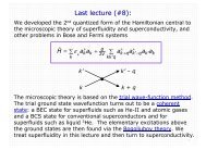
Set of supplementary notes.

You also want an ePaper? Increase the reach of your titles
YUMPU automatically turns print PDFs into web optimized ePapers that Google loves.
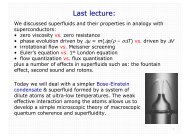
128 CHAPTER 9. ELECTRONIC INSTABILITIES<br />
Figure 9.1: The Peierls transition. The upper figure shows the familiar one-dimensional chain<br />
with lattice constant a and the corresponding lowest electronic band, plotted for momenta<br />
between 0 and π/a. In the lower figure (b) a periodic lattice modulation is introduced, with<br />
u(r) <strong>of</strong> the form <strong>of</strong> (9.2). The period is cunningly chosen to be exactly 2π/2k F , so that a band<br />
gap <strong>of</strong> amplitude 2g Q u 0 is introduced exactly at the chemical potential.<br />
in the limit u o /a ≪ 1, and A is a constant (depending on g Q ). Note the logarithm — this varies<br />
faster than quadratically (just). It is negative - the energy goes down with the distortion.<br />
By an extension <strong>of</strong> the standard band structure result, it should be clear that there is an<br />
electronic charge modulation accompanying the periodic lattice distortion - this is usually called<br />
a charge density wave (CDW).<br />
(9.3) is just the electronic contribution to the energy from those states very close to the<br />
fermi surface. But as we have argued before, it is sensible to model the other interactions<br />
between atoms just as springs, in which case we should add an elastic energy that is <strong>of</strong> the<br />
form<br />
E elastic = K(u o /a) 2 (9.4)