Set of supplementary notes.

4.3. NEARLY FREE ELECTRON THEORY 61
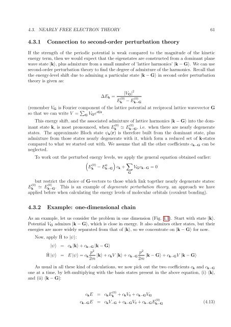
4.3.1 Connection to second-order perturbation theory
If the strength of the periodic potential is weak compared to the magnitude of the kinetic
energy term, then we would expect that the eigenstates are constructed from a dominant plane
wave state |k〉, plus admixture from a small number of ’lattice harmonics’ |k − G〉. We can use
second-order perturbation theory to find the degree of admixture of the harmonics. Recall that
the energy-level shift due to admixing a particular state |k − G〉 in second order perturbation
theory is given as:
∆E k =
E (0)
k
|V G | 2
− E(0) k−G
(remember V G is Fourier component of the lattice potential at reciprocal lattice wavevector G
so that we can write V = ∑ G V Ge iGr .
This energy shift, and the associated admixture of lattice harmonics |k − G〉 into the dominant
state k, is most pronounced, when E (0)
k
≃ E (0)
k−G
, i.e. when there are nearly degenerate
states. The approximate Bloch state ψ k (r) is therefore built from the dominant state, plus
admixture from those states nearly degenerate with it, which form a reduced set of k-states
compared to what we started out with. We assume that all the other coefficients c k−G can be
neglected.
To work out the perturbed energy levels, we apply the general equation obtained earlier:
(
)
E (0)
k
− E0 k−G c k + ∑ V G c k−G = 0
G
but restrict the choice of G-vectors to those which link together nearly degenerate states:
E (0)
k
≃ E (0)
k−G . This is an example of degenerate perturbation theory, an approach we have
applied before when calculating the energy levels of molecular orbitals (covalent bonding).
4.3.2 Example: one-dimensional chain
As an example, let us consider the problem in one dimension (Fig. 4.1). Start with state |k〉.
Potential V G admixes |k − G〉, which is close in energy. It also admixes other states, but their
energies are more widely separated from that of |k〉, so we concentrate on |k − G〉 for now.
Now, apply Ĥ to |ψ〉:
|ψ〉 = c k |k〉 + c k−G |k − G〉
Ĥ |ψ〉 =
p 2
E |ψ〉 = c k
2m |k〉 + c p 2
kV |k〉 + c k−G
2m |k − G〉 + c k−GV |k − G〉
As usual in all these kind of calculations, we now pick out the two coefficients c k and c k−G
one at a time, by left-multiplying with the basis states present in the above equation, (i) 〈k|,
and (ii) 〈k − G|:
c k E = c k E (0)
k
+ c kV 0 + c k−G V G
c k−G E = c k V −G + c k−G V 0 + c k−G E (0)
k−G
(4.13)