gas hydrate - CCOP

More documents

Recommendations

Info

Several methods for computing the Q factor, such as amplitude decay, analytical signal, wavelet modeling, rise time method, and spectral ratio have been investigated in the literature by Tonn (1991). In spite of the broad variety of methods available for computation of Q, the spectral ratio method has been widely used, especially, in obtaining Q’s from VSP data (De et al., 1994; Pramanik et al., 2000; Reid et al., 2001) because it is easier and faster to apply. To overcome the instability of the frequency-independent Q computed by the spectral ratio method, Jeng et al. (1999) introduced the modified spectral method which yields frequencydependent Q. In this study, we developed the algorithms of the spectral ratio method and the modified spectral ratio method. The developed algorithms were applied to synthetic zero-offset VSP data sets and the zero-offset VSP data acquired at Mallik 3L-38 gas hydrate production research well, and the results are analyzed. METHODS FOR COMPUTATION OF Q FACTOR Spectral Ratio Method In the spectral ratio method, the amplitude spectrum ( z f ) z is assumed to decay exponentially from a reference amplitude spectrum A ( z , f ) A , of the trace from geophone level 0 0 at a shallow level z 0 . This exponential decay can be written as A −α ( z−z0 ) ( z, f ) = A ( z0 , f ) e 0 (1) Where α is the absorption coefficient and α is related to Q and velocity V by πf ( QV ) Equation (1) can be written as ⎛ A ln ⎜ ⎝ Ao ( z, f ) ( z f ) 0 , ⎞ ⎟ = −α ⎠ = − πf ( z − z ) ( T − T ) = Slope ⋅ f 0 0 Q α = . Where T and T 0 are the P-wave (or S-wave) arrival times at geophone levels z and z 0 , respectively, and Slope is ln[ A ( z, f ) A0 ( z0 , f )] f . From equation (2), Q can be written as Q 0 ( T − T ) Slope (2) = − π . (3) We compute the Slope from a least-squares linear fit to the data points in a cross plot of ln[ A ( z, f ) A0 ( z0 , f )] versus f. The spectral ratio method assumes (De et al., 1994): 1) The source waveform is constant between upper and lower levels. 2) The geophone coupling is the same between upper and lower levels. 3) There is no interface from reflected waves. 4) There is no variation in stratigraphic filtering between upper and lower levels. 5) Q is independent of frequency in the VSP bandwidth, which means ln[ A( z, f ) A0 ( z0 , f )] = Slope ⋅ f is an equation for a straight line with a constant slope. 6) Noise is negligible. 36 New Energy Resources in the CCOP Region - Gas Hydrates and Coalbed Methane
Modified spectral ratio method To obtain an estimate of frequency dependent Q, the natural logarithm of the amplitude ratio, ln[ A ( z, f ) A0 ( z0 , f )], from equation (2) is plotted against the arrival-time difference T − of two receivers for each frequency. The slope of the regression line isπ f Q . 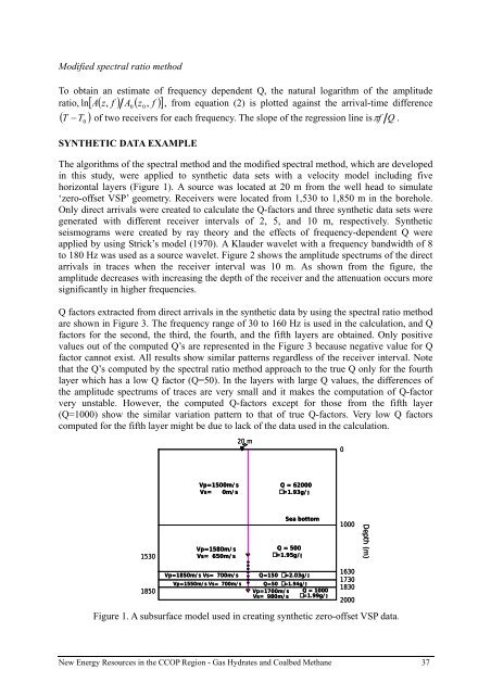( ) T 0 SYNTHETIC DATA EXAMPLE The algorithms of the spectral method and the modified spectral method, which are developed in this study, were applied to synthetic data sets with a velocity model including five horizontal layers (Figure 1). A source was located at 20 m from the well head to simulate ‘zero-offset VSP’ geometry. Receivers were located from 1,530 to 1,850 m in the borehole. Only direct arrivals were created to calculate the Q-factors and three synthetic data sets were generated with different receiver intervals of 2, 5, and 10 m, respectively. Synthetic seismograms were created by ray theory and the effects of frequency-dependent Q were applied by using Strick’s model (1970). A Klauder wavelet with a frequency bandwidth of 8 to 180 Hz was used as a source wavelet. Figure 2 shows the amplitude spectrums of the direct arrivals in traces when the receiver interval was 10 m. As shown from the figure, the amplitude decreases with increasing the depth of the receiver and the attenuation occurs more significantly in higher frequencies. Q factors extracted from direct arrivals in the synthetic data by using the spectral ratio method are shown in Figure 3. The frequency range of 30 to 160 Hz is used in the calculation, and Q factors for the second, the third, the fourth, and the fifth layers are obtained. Only positive values out of the computed Q’s are represented in the Figure 3 because negative value for Q factor cannot exist. All results show similar patterns regardless of the receiver interval. Note that the Q’s computed by the spectral ratio method approach to the true Q only for the fourth layer which has a low Q factor (Q=50). In the layers with large Q values, the differences of the amplitude spectrums of traces are very small and it makes the computation of Q-factor very unstable. However, the computed Q-factors except for those from the fifth layer (Q=1000) show the similar variation pattern to that of true Q-factors. Very low Q factors computed for the fifth layer might be due to lack of the data used in the calculation. 20 m 0 Vp=1500m/s Vs= 0m/s Q = 62000 =1.93g/ 1530 Vp=1580m/s Vs= 650m/s Sea bottom Q = 500 =1.95g/ 1000 Depth (m) 1850 Vp=1850m/s Vs= 700m/s Vp=1550m/s Vs= 700m/s Q=150 =2.03g/ Q=50 =1.94g/ Vp=1700m/s Q = 1000 Vs= 980m/s =1.99g/ 1630 1730 1830 2000 Figure 1. A subsurface model used in creating synthetic zero-offset VSP data. New Energy Resources in the CCOP Region - Gas Hydrates and Coalbed Methane 37
Page 2 and 3: Coordinating Committee for Geoscien
Page 4 and 5: Thematic Session on New Energy Reso
Page 6 and 7: CONTENTS Page OPENING REMARKS……
Page 8 and 9: OPENING REMARKS by Chen Shik Pei Di
Page 10 and 11: WELCOME ADDRESS by Tai-Sup Lee Pres
Page 12 and 13: WELCOME ADDRESS by Keun-Pil Park Di
Page 14 and 15: CONGRATULATORY ADDRESS by David Pri
Page 16 and 17: PART I GAS HYDRATE: EXPLORATION, RE
Page 18 and 19: Partial differential equations for
Page 20 and 21: RESULTS AND DISCUSSION In the follo
Page 22 and 23: REFERENCES Berner R. A. (1980) Earl
Page 24 and 25: features of the seabed than those o
Page 26 and 27: secure the stability of the solutio
Page 28 and 29: trends depending on the following f
Page 30 and 31: Organic carbon in sediments is of i
Page 32 and 33: Sedimentological and Geochemical As
Page 34 and 35: Figure 3. Sedimentation rate of the
Page 36 and 37: Marine Gas Hydrate off W. Canada an
Page 40 and 41: 0.035 0.03 Amplitude 0.025 0.02 0.0
Page 42 and 43: 60 50 Amplitude 40 30 20 10 0 0 50
Page 44 and 45: REFERENCES Dallimore, S.R. and T.S.
Page 46 and 47: Frequency % 20 16 12 8 HAMA #5, MV=
Page 48 and 49: Figure 3. Experimental procedures f
Page 50 and 51: Figure 7 shows two cases of the com
Page 52 and 53: Seismic Characteristics of Gas Hydr
Page 54 and 55: Purpose The purpose of this paper i
Page 56 and 57: The dissociation zone created by th
Page 58 and 59: hydrate that forms near the wellbor
Page 60 and 61: dissociation, composite thermal con
Page 62 and 63: Figure 9. The Advanced Light Source
Page 64 and 65: Experimental Studies and Developmen
Page 66 and 67: Natural gas hydrate exploitation an
Page 68 and 69: Natural gas Free gas layer Figure 5
Page 70 and 71: Figure 7. One-dimensional developme
Page 72 and 73: Temper at ur e 2 1 0 -1 -2 -3 -4
Page 74 and 75: From the above discussion, the heat
Page 76 and 77: INTRODUCTION Clathrate hydrates are
Page 78 and 79: MATHEMATICAL MODEL The mathematical
Page 80 and 81: Where the hydrate-aqueous radius of
Page 82 and 83: REFERENCES Brooks, R.H., and A.T. C
Page 84 and 85: 86 New Energy Resources in the CCOP
Page 86 and 87: In this paper, an overview of the M
Page 88 and 89:
The brief tasks in the Phase I are:
Page 90 and 91:
In "Development of the dissociation
Page 92 and 93:
Figure 5. Preparation equipment. AN
Page 94 and 95:
Other recent research subjects in t
Page 96 and 97:
same crystalline structure directly
Page 98 and 99:
Another important aspect of the pre
Page 100 and 101:
a + CO 2 CH 4 C 2 H 6 b CH 4 in sII
Page 102 and 103:
REFERENCES Collett, T.S. and Kuuskr
Page 104 and 105:
Figure 1. Physiographic and crust m
Page 106 and 107:
Figure 3. Seismic profile showing s
Page 108 and 109:
Figure 7. Distribution of echo char
Page 110 and 111:
Figure 10. Seismic profile and its
Page 112 and 113:
In the early stage of back-arc open
Page 114 and 115:
PART II COALBED METHANE (CBM)
Page 116 and 117:
Supply and demand infrastructure of
Page 118 and 119:
Amisan, Jogyeri, Baegunsa, and Seon
Page 120 and 121:
PROPERTIES OF ANTHRACITE The coals
Page 122 and 123:
Table 4. Average chemical compositi
Page 124 and 125:
CONCLUSIONS 1. Most of the coals em
Page 126 and 127:
INTRODUCTION Coal (total reserves 2
Page 128 and 129:
ีีีีีีีีี ั ิ
Page 130 and 131:
RESULTS By Government: The outcomes
Page 132 and 133:
The gas composition (12 samples ana
Page 134 and 135:
Table 4. Coal Depth Interval Hole N
Page 136 and 137:
The results of studies made on 11 c
Page 138 and 139:
CONCLUSION CBM is still hoped to be
Page 140 and 141:
The Government of Indonesia through
Page 142 and 143:
The Berau basin is a major coal pro
Page 144 and 145:
PP: CBM - 1 Rambutan (GOI Sponsor)
Page 146 and 147:
Overview of Project for CO 2 Seques
Page 148 and 149:
The organic geochemistry research g
Page 150 and 151:
3.5 25 3.0 20 Ar(%) C O 2(%) 2.5 2
Page 152 and 153:
20 8 10 0 6 δ13C of CO2(‰) -10 -
Page 154 and 155:
Figure 1. Index map of Akabira Coal
Page 156:
ORIGIN OF AKABIRA CBM In Akabira mi
show all

gas hydrate - CCOP

You also want an ePaper? Increase the reach of your titles

Delete template?

Save as template?