CEIOPS' Advice for Level 2 Implementing ... - EIOPA - Europa
CEIOPS' Advice for Level 2 Implementing ... - EIOPA - Europa
CEIOPS' Advice for Level 2 Implementing ... - EIOPA - Europa

Create successful ePaper yourself
Turn your PDF publications into a flip-book with our unique Google optimized e-Paper software.
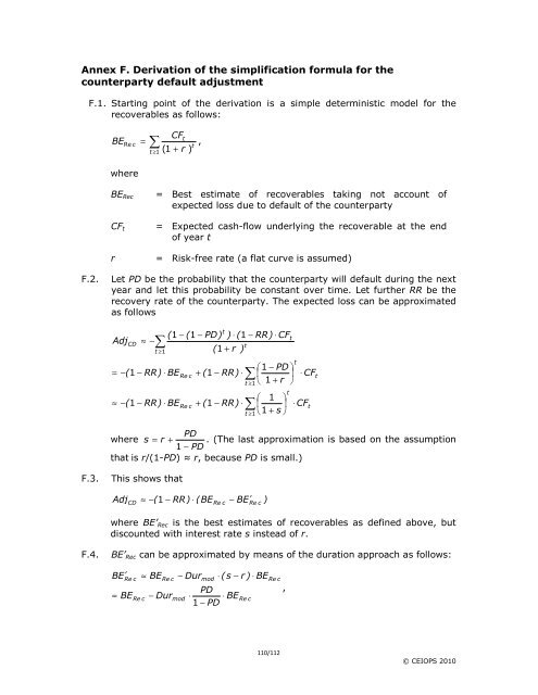
Annex F. Derivation of the simplification <strong>for</strong>mula <strong>for</strong> the<br />
counterparty default adjustment<br />
F.1. Starting point of the derivation is a simple deterministic model <strong>for</strong> the<br />
recoverables as follows:<br />
CFt<br />
BE Re c =<br />
, t<br />
( 1 + r )<br />
where<br />
BERec<br />
CFt<br />
∑<br />
t ≥ 1<br />
= Best estimate of recoverables taking not account of<br />
expected loss due to default of the counterparty<br />
= Expected cash-flow underlying the recoverable at the end<br />
of year t<br />
r = Risk-free rate (a flat curve is assumed)<br />
F.2. Let PD be the probability that the counterparty will default during the next<br />
year and let this probability be constant over time. Let further RR be the<br />
recovery rate of the counterparty. The expected loss can be approximated<br />
as follows<br />
Adj<br />
CD<br />
≈ −<br />
∑<br />
t ≥1<br />
= −(<br />
1 − RR)<br />
≈ −(<br />
1 − RR)<br />
( 1 − ( 1 − PD)<br />
) ⋅ ( 1 − RR)<br />
⋅ CF<br />
⋅ BE<br />
⋅ BE<br />
Re c<br />
Re c<br />
+ ( 1 − RR)<br />
+ ( 1 − RR)<br />
t<br />
( 1 + r )<br />
⋅<br />
⋅<br />
t<br />
∑<br />
t ≥1<br />
∑<br />
t ≥1<br />
⎛1<br />
− PD ⎞<br />
⎜ ⎟ ⋅ CFt<br />
⎝ 1 + r ⎠<br />
⎛ 1 ⎞<br />
⎜ ⎟<br />
⎝1<br />
+ s ⎠<br />
110/112<br />
t<br />
t<br />
t<br />
⋅ CF<br />
PD<br />
where s = r + . (The last approximation is based on the assumption<br />
1 − PD<br />
that is r/(1-PD) ≈ r, because PD is small.)<br />
F.3. This shows that<br />
AdjCD ≈ −(<br />
1 − RR)<br />
⋅ ( BERe<br />
c − BERe<br />
′ c )<br />
where BE’Rec is the best estimates of recoverables as defined above, but<br />
discounted with interest rate s instead of r.<br />
F.4. BE’Rec can be approximated by means of the duration approach as follows:<br />
BE<br />
′<br />
Re c<br />
= BE<br />
Re c<br />
≈ BE<br />
Re c<br />
− Dur<br />
− Dur<br />
mod<br />
mod<br />
PD<br />
⋅ ⋅ BE<br />
1 − PD<br />
⋅ ( s − r ) ⋅ BE<br />
Re c<br />
Re c<br />
,<br />
t<br />
© CEIOPS 2010