Here - Stuff

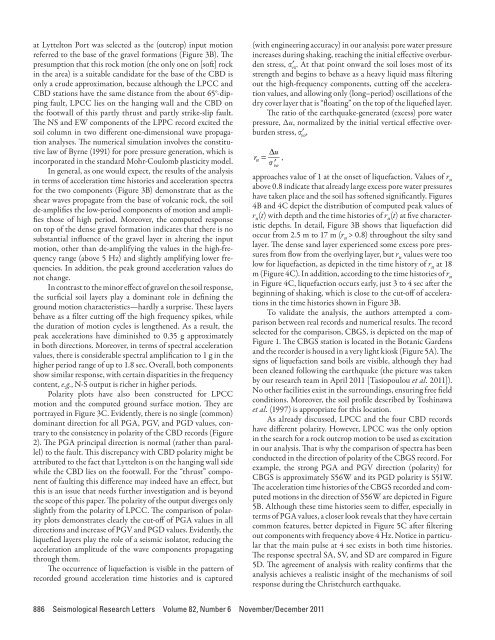
at Lyttelton Port was selected as the (outcrop) input motionreferred to the base of the gravel formations (Figure 3B). Thepresumption that this rock motion (the only one on [soft] rockin the area) is a suitable candidate for the base of the CBD isonly a crude approximation, because although the LPCC andCBD stations have the same distance from the about 65°-dippingfault, LPCC lies on the hanging wall and the CBD onthe footwall of this partly thrust and partly strike-slip fault.The NS and EW components of the LPPC record excited thesoil column in two different one-dimensional wave propagationanalyses. The numerical simulation involves the constitutivelaw of Byrne (1991) for pore pressure generation, which isincorporated in the standard Mohr-Coulomb plasticity model.In general, as one would expect, the results of the analysisin terms of acceleration time histories and acceleration spectrafor the two components (Figure 3B) demonstrate that as theshear waves propagate from the base of volcanic rock, the soilde-amplifies the low-period components of motion and amplifiesthose of high period. Moreover, the computed responseon top of the dense gravel formation indicates that there is nosubstantial influence of the gravel layer in altering the inputmotion, other than de-amplifying the values in the high-frequencyrange (above 5 Hz) and slightly amplifying lower frequencies.In addition, the peak ground acceleration values donot change.In contrast to the minor effect of gravel on the soil response,the surficial soil layers play a dominant role in defining theground motion characteristics—hardly a surprise. These layersbehave as a filter cutting off the high frequency spikes, whilethe duration of motion cycles is lengthened. As a result, thepeak accelerations have diminished to 0.35 g approximatelyin both directions. Moreover, in terms of spectral accelerationvalues, there is considerable spectral amplification to 1 g in thehigher period range of up to 1.8 sec. Overall, both componentsshow similar response, with certain disparities in the frequencycontent, e.g., N-S output is richer in higher periods.Polarity plots have also been constructed for LPCCmotion and the computed ground surface motion. They areportrayed in Figure 3C. Evidently, there is no single (common)dominant direction for all PGA, PGV, and PGD values, contraryto the consistency in polarity of the CBD records (Figure2). The PGA principal direction is normal (rather than parallel)to the fault. This discrepancy with CBD polarity might beattributed to the fact that Lyttelton is on the hanging wall sidewhile the CBD lies on the footwall. For the “thrust” componentof faulting this difference may indeed have an effect, butthis is an issue that needs further investigation and is beyondthe scope of this paper. The polarity of the output diverges onlyslightly from the polarity of LPCC. The comparison of polarityplots demonstrates clearly the cut-off of PGA values in alldirections and increase of PGV and PGD values. Evidently, theliquefied layers play the role of a seismic isolator, reducing theacceleration amplitude of the wave components propagatingthrough them.The occurrence of liquefaction is visible in the pattern ofrecorded ground acceleration time histories and is captured(with engineering accuracy) in our analysis: pore water pressureincreases during shaking, reaching the initial effective overburdenstress, σ′ νο . At that point onward the soil loses most of itsstrength and begins to behave as a heavy liquid mass filteringout the high-frequency components, cutting off the accelerationvalues, and allowing only (long–period) oscillations of thedry cover layer that is “floating” on the top of the liquefied layer.The ratio of the earthquake-generated (excess) pore waterpressure, Δu, normalized by the initial vertical effective overburdenstress, σ′ νo ,r u =uσ νo,approaches value of 1 at the onset of liquefaction. Values of r uabove 0.8 indicate that already large excess pore water pressureshave taken place and the soil has softened significantly. Figures4B and 4C depict the distribution of computed peak values ofr u (t) with depth and the time histories of r u (t) at five characteristicdepths. In detail, Figure 3B shows that liquefaction didoccur from 2.5 m to 17 m (r u > 0.8) throughout the silty sandlayer. The dense sand layer experienced some excess pore pressuresfrom flow from the overlying layer, but r u values were toolow for liquefaction, as depicted in the time history of r u at 18m (Figure 4C). In addition, according to the time histories of r uin Figure 4C, liquefaction occurs early, just 3 to 4 sec after thebeginning of shaking, which is close to the cut-off of accelerationsin the time histories shown in Figure 3B.To validate the analysis, the authors attempted a comparisonbetween real records and numerical results. The recordselected for the comparison, CBGS, is depicted on the map ofFigure 1. The CBGS station is located in the Botanic Gardensand the recorder is housed in a very light kiosk (Figure 5A). Thesigns of liquefaction sand boils are visible, although they hadbeen cleaned following the earthquake (the picture was takenby our research team in April 2011 [Tasiopoulou et al. 2011]).No other facilities exist in the surroundings, ensuring free fieldconditions. Moreover, the soil profile described by Toshinawaet al. (1997) is appropriate for this location.As already discussed, LPCC and the four CBD recordshave different polarity. However, LPCC was the only optionin the search for a rock outcrop motion to be used as excitationin our analysis. That is why the comparison of spectra has beenconducted in the direction of polarity of the CBGS record. Forexample, the strong PGA and PGV direction (polarity) forCBGS is approximately S56W and its PGD polarity is S51W.The acceleration time histories of the CBGS recorded and computedmotions in the direction of S56W are depicted in Figure5B. Although these time histories seem to differ, especially interms of PGA values, a closer look reveals that they have certaincommon features, better depicted in Figure 5C after filteringout components with frequency above 4 Hz. Notice in particularthat the main pulse at 4 sec exists in both time histories.The response spectral SA, SV, and SD are compared in Figure5D. The agreement of analysis with reality confirms that theanalysis achieves a realistic insight of the mechanisms of soilresponse during the Christchurch earthquake.886 Seismological Research Letters Volume 82, Number 6 November/December 2011