Here - Stuff

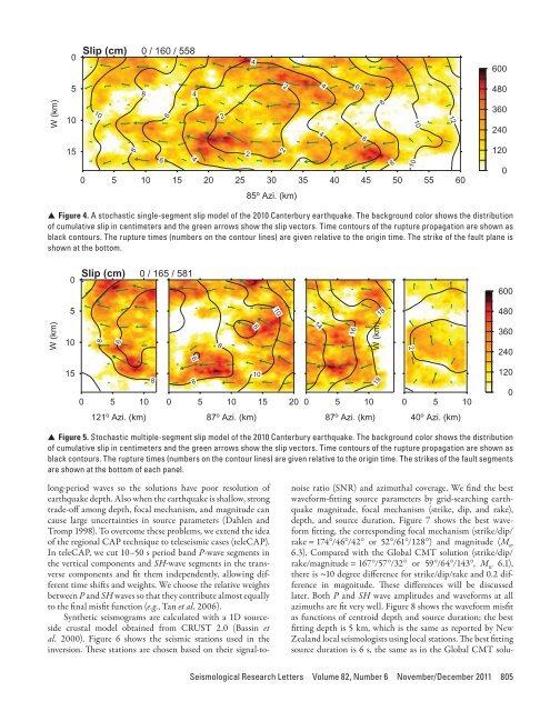
0Slip (cm) 0 / 160 / 55846005842464808W (km)1015108664220 5 10 15 20 25 30 35 40 45 50 55 602468101012360240120085 o Azi. (km)▲▲Figure 4. A stochastic single-segment slip model of the 2010 Canterbury earthquake. The background color shows the distributionof cumulative slip in centimeters and the green arrows show the slip vectors. Time contours of the rupture propagation are shown asblack contours. The rupture times (numbers on the contour lines) are given relative to the origin time. The strike of the fault plane isshown at the bottom.0Slip (cm) 0 / 165 / 58160051018480W (km)10866881416W (km)2360240150 5 1088100 5 10 15 200 5 10180 5 101200121 o Azi. (km)87 o Azi. (km)87 o Azi. (km)40 o Azi. (km)▲ ▲ Figure 5. Stochastic multiple-segment slip model of the 2010 Canterbury earthquake. The background color shows the distributionof cumulative slip in centimeters and the green arrows show the slip vectors. Time contours of the rupture propagation are shown asblack contours. The rupture times (numbers on the contour lines) are given relative to the origin time. The strikes of the fault segmentsare shown at the bottom of each panel.long-period waves so the solutions have poor resolution ofearthquake depth. Also when the earthquake is shallow, strongtrade-off among depth, focal mechanism, and magnitude cancause large uncertainties in source parameters (Dahlen andTromp 1998). To overcome these problems, we extend the ideaof the regional CAP technique to teleseismic cases (teleCAP).In teleCAP, we cut 10–50 s period band P-wave segments inthe vertical components and SH-wave segments in the transversecomponents and fit them independently, allowing differenttime shifts and weights. We choose the relative weightsbetween P and SH waves so that they contribute almost equallyto the final misfit function (e.g., Tan et al. 2006).Synthetic seismograms are calculated with a 1D sourcesidecrustal model obtained from CRUST 2.0 (Bassin etal. 2000). Figure 6 shows the seismic stations used in theinversion. These stations are chosen based on their signal-tonoiseratio (SNR) and azimuthal coverage. We find the bestwaveform-fitting source parameters by grid-searching earthquakemagnitude, focal mechanism (strike, dip, and rake),depth, and source duration. Figure 7 shows the best waveformfitting, the corresponding focal mechanism (strike/dip/rake = 174°/46°/42° or 52°/61°/128°) and magnitude (M w6.3). Compared with the Global CMT solution (strike/dip/rake/magnitude = 167°/57°/32° or 59°/64°/143°, M w 6.1),there is ~10 degree difference for strike/dip/rake and 0.2 differencein magnitude. These differences will be discussedlater. Both P and SH wave amplitudes and waveforms at allazimuths are fit very well. Figure 8 shows the waveform misfitas functions of centroid depth and source duration; the bestfitting depth is 5 km, which is the same as reported by NewZealand local seismologists using local stations. The best fittingsource duration is 6 s, the same as in the Global CMT solu-Seismological Research Letters Volume 82, Number 6 November/December 2011 805