Here - Stuff

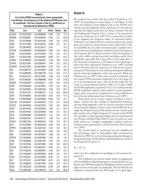
TABLE 1List of the HVSR measurements, their geographiccoordinates, the frequency of the highest HVSR peak andits amplitude. The last column is the K g coefficient asintroduced by Nakamura (1996).Site Lon Lat Fmax Amax KgCACS 172.5275768 –43.4826609 5.88 2.8 1.3RSMC 172.5628001 –43.5355676 0.94 3.2 10.9N13 172.5705568 –43.5437258 2.00 5.0 12.5N26 172.5777560 –43.5108726 3.88 3.7 3.5N27 172.5818618 –43.5213617 3.19 2.5PPHS 172.6064083 –43.4936198 2.06 5.9 16.9N28 172.6125849 –43.5122464 1.81 3.2 5.7N25 172.6167294 –43.5493591 0.50 3.1 19.2CBGS 172.6199070 –43.5292657 1.38 4.0 11.6CHHC 172.6234361 –43.5368474 1.44 3.5 8.5CMHS 172.6273183 –43.5675024 3.75 4.5 5.4N3 172.6306775 –43.5275045 2.06 4.5 9.8N2 172.6306950 –43.5285730 2.13 5.0 11.7N1 172.6313143 –43.5311002 1.46 4.0 11.0N12 172.6346267 –43.5806096 0.81 3.8 17.8RHES 172.6354074 –43.5235211 2.05 6.0 17.6N30 172.6355683 –43.5310515 1.50 3.9 10.1N32 172.6355845 –43.5284343 1.50 5.0 16.7N31 172.6413124 –43.5309137 1.75 6.0 20.6N14 172.6416583 –43.5213395 2.25 5.0 11.1N24 172.6429684 –43.5476508 0.69 2.5 9.1N4-N5 172.6458412 –43.5257455 1.75 4.3 10.6CCCC 172.6461493 –43.5373261 1.50 4.9 16.0N29 172.6473579 –43.4943542 1.56 5.1 16.7N15 172.6519704 –43.5319409 1.63 3.7 8.4N10 172.6596168 –43.5500570 1.13 4.4 17.1N16 172.6642247 –43.5319177 1.38 2.2 3.5SHLC 172.6651345 –43.5040313 1.50 2.5 4.2N11 172.6752989 –43.5624248 2.63 4.0 6.1PRPC 172.6823280 –43.5281150 1.25 3.4 9.2N17 172.6874653 –43.5401185 1.63 2.8 4.8N6 172.6879189 –43.5015612 1.80 2.2 2.7HPSC 172.7019825 –43.5024466 1.25 1.5 1.8N18 172.7049053 –43.5361145 1.94 2.8 4.0N21 172.7071643 –43.5575285 1.55 5.6 20.2HVSC 172.7082133 –43.5807977 3.56 4.2 5.0N9 172.7228573 –43.6046841 7.44 6.2 5.2N8 172.7233046 –43.6033945 6.06 3.4 1.9N19 172.7291321 –43.5239186 0.38 1.7 7.6N7 172.7313212 –43.5077893 0.31 2.2 15.6N23 172.7360934 –43.5611169 2.00 4.5 10.1N20 172.7433333 –43.5401993 0.50 3.8 28.9N22 172.7604590 –43.5769734 1.25 9.8 76.8RESULTSWe compared our results with the results of Toshinawa et al.(1997) by preparing two maps (Figure 2 and Figure 3) thatshow the frequency of the highest peak in the HVSR curveand the relevant amplitude (Fmax and Amax). It is worth notingthat this highest peak does not always coincide with thesoil fundamental frequency but is closer to the parameterschosen by Toshinawa et al. (1997), for a reason that is evidentif one compares the frequency maps. As mentioned before,Toshinawa et al. did not find any resonance peak in the coastaldune area, while our measurements return values below 1 Hz.It is probable that the older instrumentation, coupled with ashorter-duration sampling time, could not detect low frequencysoil resonance due to a deeper structure. This low frequency isalso often visible moving westward, providing a peak whoseamplitude is generally lower than those in the range above 1Hz. The peaks at frequency >1 Hz appear to be in good agreementwith those reported by Toshinawa et al. (1997), passingfrom 1 Hz below the city center up to 5–6 Hz in the westernmostpart of Christchurch. Our results present quite a differentpicture when the amplitude is taken into account. While theToshinawa et al. (1997) values never exceed 6 and below thecity center HVSR maximum amplitudes are in the range of 2to 3, our measurements top a value of 10 and under the citycenter (or central business district, CBD, as it is often called)the HVSR amplitudes range from 3.5 to 7. It is well known thatHVSR amplitude could be rather sensitive to processing techniques,and a more precise comparison was not possible due tolack of further information from Toshinawa et al. (1997).More detail on our results is given in Figures 4 and 5.Figure 4 shows the clear change in fundamental frequencymoving along longitude, with an increase moving westward.The second plot (Figure 5) shows a site with HVSR that has asingle, low-frequency peak while another site has a similar peakplus another one at higher frequency. It is known that HVSRhas a problem in showing modes higher than the fundamentalone (Parolai and Richwalski 2004), so the two peaks are mostlikely related to a complex stratigraphic situation with tworesonant strata separated by a velocity inversion (Di Giacomoet al. 2005).The second check we performed was the reliability ofthe soil damage index or vulnerability index introduced byNakamura (1996) for use in estimating earthquake damage onthe ground surface. Its distribution should delineate weak areason the ground. It is given as:K g = A g 2 / F g ,where A g is the amplitude corresponding to soil resonance frequencyF g .This coefficient was used in studies aimed at mapping thesoil susceptibility to liquefaction prior to an earthquake (see, e.g.,Beroya et al. 2009 for Laoag City, Philippines), but to our knowledgewas never tested after an earthquake. The fact that the soilfrequencies measured after the 2011 quake are in good agree-920 Seismological Research Letters Volume 82, Number 6 November/December 2011