The Genom of Homo sapiens.pdf

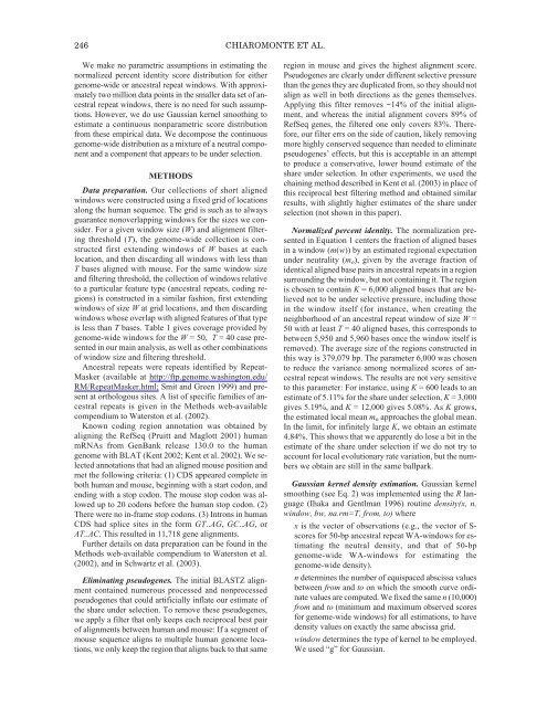
246 CHIAROMONTE ET AL.We make no parametric assumptions in estimating thenormalized percent identity score distribution for eithergenome-wide or ancestral repeat windows. With approximatelytwo million data points in the smaller data set of ancestralrepeat windows, there is no need for such assumptions.However, we do use Gaussian kernel smoothing toestimate a continuous nonparametric score distributionfrom these empirical data. We decompose the continuousgenome-wide distribution as a mixture of a neutral componentand a component that appears to be under selection.METHODSData preparation. Our collections of short alignedwindows were constructed using a fixed grid of locationsalong the human sequence. The grid is such as to alwaysguarantee nonoverlapping windows for the sizes we consider.For a given window size (W) and alignment filteringthreshold (T), the genome-wide collection is constructedfirst extending windows of W bases at eachlocation, and then discarding all windows with less thanT bases aligned with mouse. For the same window sizeand filtering threshold, the collection of windows relativeto a particular feature type (ancestral repeats, coding regions)is constructed in a similar fashion, first extendingwindows of size W at grid locations, and then discardingwindows whose overlap with aligned features of that typeis less than T bases. Table 1 gives coverage provided bygenome-wide windows for the W = 50, T = 40 case presentedin our main analysis, as well as other combinationsof window size and filtering threshold.Ancestral repeats were repeats identified by Repeat-Masker (available at http://ftp.genome.washington.edu/RM/RepeatMasker.html; Smit and Green 1999) and presentat orthologous sites. A list of specific families of ancestralrepeats is given in the Methods web-availablecompendium to Waterston et al. (2002).Known coding region annotation was obtained byaligning the RefSeq (Pruitt and Maglott 2001) humanmRNAs from GenBank release 130.0 to the humangenome with BLAT (Kent 2002; Kent et al. 2002). We selectedannotations that had an aligned mouse position andmet the following criteria: (1) CDS appeared complete inboth human and mouse, beginning with a start codon, andending with a stop codon. The mouse stop codon was allowedup to 20 codons before the human stop codon. (2)There were no in-frame stop codons. (3) Introns in humanCDS had splice sites in the form GT..AG, GC..AG, orAT..AC. This resulted in 11,718 gene alignments.Further details on data preparation can be found in theMethods web-available compendium to Waterston et al.(2002), and in Schwartz et al. (2003).Eliminating pseudogenes. The initial BLASTZ alignmentcontained numerous processed and nonprocessedpseudogenes that could artificially inflate our estimate ofthe share under selection. To remove these pseudogenes,we apply a filter that only keeps each reciprocal best pairof alignments between human and mouse: If a segment ofmouse sequence aligns to multiple human genome locations,we only keep the region that aligns back to that sameregion in mouse and gives the highest alignment score.Pseudogenes are clearly under different selective pressurethan the genes they are duplicated from, so they should notalign as well in both directions as the genes themselves.Applying this filter removes ~14% of the initial alignment,and whereas the initial alignment covers 89% ofRefSeq genes, the filtered one only covers 83%. Therefore,our filter errs on the side of caution, likely removingmore highly conserved sequence than needed to eliminatepseudogenes’ effects, but this is acceptable in an attemptto produce a conservative, lower bound estimate of theshare under selection. In other experiments, we used thechaining method described in Kent et al. (2003) in place ofthis reciprocal best filtering method and obtained similarresults, with slightly higher estimates of the share underselection (not shown in this paper).Normalized percent identity. The normalization presentedin Equation 1 centers the fraction of aligned basesin a window (m(w)) by an estimated regional expectationunder neutrality (m o ), given by the average fraction ofidentical aligned base pairs in ancestral repeats in a regionsurrounding the window, but not containing it. The regionis chosen to contain K = 6,000 aligned bases that are believednot to be under selective pressure, including thosein the window itself (for instance, when creating theneighborhood of an ancestral repeat window of size W =50 with at least T = 40 aligned bases, this corresponds tobetween 5,950 and 5,960 bases once the window itself isremoved). The average size of the regions constructed inthis way is 379,079 bp. The parameter 6,000 was chosento reduce the variance among normalized scores of ancestralrepeat windows. The results are not very sensitiveto this parameter: For instance, using K = 600 leads to anestimate of 5.11% for the share under selection, K = 3,000gives 5.19%, and K = 12,000 gives 5.08%. As K grows,the estimated local mean m o approaches the global mean.In the limit, for infinitely large K, we obtain an estimate4.84%. This shows that we apparently do lose a bit in theestimate of the share under selection if we do not try toaccount for local evolutionary rate variation, but the numberswe obtain are still in the same ballpark.Gaussian kernel density estimation. Gaussian kernelsmoothing (see Eq. 2) was implemented using the R language(Ihaka and Gentlman 1996) routine density(x, n,window, bw, na.rm=T, from, to) where• x is the vector of observations (e.g., the vector of S-scores for 50-bp ancestral repeat WA-windows for estimatingthe neutral density, and that of 50-bpgenome-wide WA-windows for estimating thegenome-wide density).• n determines the number of equispaced abscissa valuesbetween from and to on which the smooth curve ordinatevalues are computed. We fixed the same n (10,000)from and to (minimum and maximum observed scoresfor genome-wide windows) for all estimations, to havedensity values on exactly the same abscissa grid.• window determines the type of kernel to be employed.We used “g” for Gaussian.